




Cell-type proportions for every bin of million-bin spatial transcriptomics.
FlashDeconv estimates the cell-type composition of each spot or bin in spatial transcriptomics data (Visium, Visium HD, Stereo-seq) from a single-cell reference.
- Fast: one million Visium HD bins in about 40 seconds on a CPU node.
- Accurate: ranks first of 13 methods on the Spotless benchmark and stays accurate as bins become sparse.
- Deterministic: the same data and reference always give the same proportions.
- Self-checking: flags tissue that the reference cannot explain and names the missing cell types.
pip install "flashdeconv[io,scanpy]"Requires Python 3.9–3.14. The core package (pip install flashdeconv) needs only NumPy, SciPy and Numba; the io and scanpy extras add AnnData support.
import scanpy as sc
import flashdeconv as fd

adata_st = sc.read_h5ad("spatial.h5ad")      # raw counts, coordinates in .obsm["spatial"]
adata_ref = sc.read_h5ad("reference.h5ad")   # raw counts, labels in .obs["cell_type"]

fd.tl.deconvolve(adata_st, adata_ref, cell_type_key="cell_type")

proportions = adata_st.obsm["flashdeconv"]   # locations × cell types, rows sum to 1
Shared genes are matched by name. If counts are stored in layers, pass layer_st="counts" and layer_ref="counts". FlashDeconv is also available in ChatSpatial, which runs spatial analyses through natural language.
A reference that lacks a cell type present in the tissue forces the model to explain those transcripts with the wrong types. The reference diagnostic scores every bin for counts that no mixture of reference profiles can explain, and reports the genes behind the misfit:
from flashdeconv import FlashDeconv, reference_fit_scores, unexplained_genes
from flashdeconv.io import prepare_data

Y, X, coords, cell_types, genes = prepare_data(adata_st, adata_ref, cell_type_key="cell_type")
model = FlashDeconv().fit(Y, X, coords, cell_type_names=cell_types)

scores = reference_fit_scores(model)
flagged = scores["flag_pooled"]               # bins the reference cannot explain
print(f"{flagged.mean():.1%} of bins flagged (about 5% expected by chance)")

top = unexplained_genes(model, flagged, gene_names=genes)
print(top["gene"][:20])                       # markers of the missing cell types
A flagged fraction well above 5%, concentrated in coherent regions, points to a missing lineage; the unexplained genes identify it. suggest_missing_types ranks candidate types from a broader atlas.
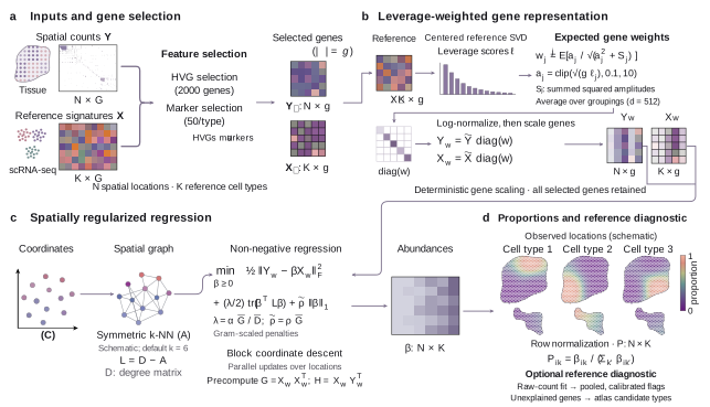
-
Genes. Select highly variable genes of the spatial data together with marker genes of each reference cell type, and log-normalize both datasets (counts per 10,000,
log1p). -
Weights. Weight each gene by its leverage score in the reference, a measure of how strongly it separates cell types. Discriminative genes dominate the fit, which keeps sparse bins accurate.
-
Regression. Fit non-negative abundances with a sparse spatial-graph penalty that shares information between neighbouring bins and an L1 penalty that favours sparse compositions:
minimize ½‖Y_w − β X_w‖² + ½ λ Tr(βᵀ L β) + ρ ‖β‖₁ subject to β ≥ 0Y_w(bins × genes) andX_w(cell types × genes) are the weighted data and reference, andLis the Laplacian of a k-nearest-neighbour graph. Both penalties are scaled automatically. -
Proportions. Normalize each row of β to obtain cell-type proportions.
A block coordinate descent solver updates all bins in parallel; its cost grows linearly with the number of bins.
Speed on real Visium HD colorectal cancer bins (18,082 genes, 38 cell types, 32 CPU threads):
| Bins | Time | Peak memory |
|---|---|---|
| 10,000 | 1.9 s | 1.9 GB |
| 100,000 | 5.4 s | 2.7 GB |
| 1,000,000 | 40 s | 12.6 GB |
Accuracy on the 54 silver-standard datasets of the Spotless benchmark (mean Pearson correlation with the true proportions):
| FlashDeconv | RCTD | Cell2location |
|---|---|---|
| 0.946 | 0.934 | 0.918 |
Benchmark details and analysis scripts are in the manuscript scripts repository.
AnnData: fd.tl.deconvolve(adata_st, adata_ref, cell_type_key=...) stores proportions in adata_st.obsm["flashdeconv"] and the dominant type in adata_st.obs["flashdeconv_dominant"].
NumPy: provide spatial counts Y (bins × genes, dense or sparse), reference signatures X (cell types × genes, mean counts per type) with the same genes in the same order, and coordinates coords (bins × 2 or 3):
from flashdeconv import FlashDeconv

model = FlashDeconv()
proportions = model.fit_transform(Y, X, coords)| Parameter | Default | Description |
|---|---|---|
lambda_spatial |
"auto" |
Spatial regularization strength |
rho_sparsity |
0.01 |
L1 sparsity strength |
n_hvg |
2000 |
Highly variable genes |
n_markers_per_type |
50 |
Marker genes per cell type |
spatial_method |
"knn" |
Spatial graph: "knn", "radius" or "grid" |
k_neighbors |
6 |
Neighbours in the k-NN graph |
max_iter, tol |
1000, 1e-4 |
Solver iteration limit and convergence tolerance |
After fitting, model.proportions_ holds the proportions, model.beta_ the unnormalized abundances and model.info_ convergence information. Uncertainty estimates (compute_uncertainty, bootstrap_uncertainty) are model-based and reflect sampling noise under the fitted model. The API reference documents all parameters and functions.
- Reference. Include every cell type expected in the tissue and check with the reference diagnostic. Merge subtypes whose profiles are nearly identical.
- Single-cell platforms. For segmented data such as Xenium, set
lambda_spatial=0or aggregate cells into multi-cell bins. - Stereo-seq. See the Stereo-seq guide.
Yang, C., Chen, J. & Zhang, X. FlashDeconv reveals resolution horizons in atlas-scale spatial transcriptomics. bioRxiv (2025). doi:10.64898/2025.12.22.696108
@article{yang2025flashdeconv,
  title   = {FlashDeconv reveals resolution horizons in atlas-scale spatial transcriptomics},
  author  = {Yang, Chen and Chen, Jun and Zhang, Xianyang},
  journal = {bioRxiv},
  year    = {2025},
  doi     = {10.64898/2025.12.22.696108}
}
To cite a specific software version, use its Zenodo DOI.
BSD 3-Clause; see LICENSE. Questions and bug reports: GitHub Issues.