Category Archive

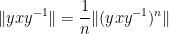
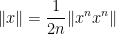
You are currently browsing the category archive for the ‘math.MG’ category.

Mathematical exploration and discovery at scale

5 November, 2025 in math.CA, math.CO, math.MG, paper | Tags: Adam Zsolt Wagner, AlphaEvolve, Artificial Intelligence, Bogdan Georgiev, Javier Gomez-Serrano, optimization | by Terence Tao | 64 comments

Bogdan Georgiev, Javier Gómez-Serrano, Adam Zsolt Wagner, and I have uploaded to the arXiv our paper “Mathematical exploration and discovery at scale“. This is a longer report on the experiments we did in collaboration with Google Deepmind with their AlphaEvolve tool, which is in the process of being made available for broader use. Some of our experiments were already reported on in a previous white paper, but the current paper provides more details, as well as a link to a repository with various relevant data such as the prompts used and the evolution of the tool outputs.

AlphaEvolve is a variant of more traditional optimization tools that are designed to extremize some given score function over a high-dimensional space of possible inputs. A traditional optimization algorithm might evolve one or more trial inputs over time by various methods, such as stochastic gradient descent, that are intended to locate increasingly good solutions while trying to avoid getting stuck at local extrema. By contrast, AlphaEvolve does not evolve the score function inputs directly, but uses an LLM to evolve computer code (often written in a standard language such as Python) which will in turn be run to generate the inputs that one tests the score function on. This reflects the belief that in many cases, the extremizing inputs will not simply be an arbitrary-looking string of numbers, but will often have some structure that can be efficiently described, or at least approximated, by a relatively short piece of code. The tool then works with a population of relatively successful such pieces of code, with the code from one generation of the population being modified and combined by the LLM based on their performance to produce the next generation. The stochastic nature of the LLM can actually work in one’s favor in such an evolutionary environment: many “hallucinations” will simply end up being pruned out of the pool of solutions being evolved due to poor performance, but a small number of such mutations can add enough diversity to the pool that one can break out of local extrema and discover new classes of viable solutions. The LLM can also accept user-supplied “hints” as part of the context of the prompt; in some cases, even just uploading PDFs of relevant literature has led to improved performance by the tool. Since the initial release of AlphaEvolve, similar tools have been developed by others, including OpenEvolve, ShinkaEvolve and DeepEvolve.

We tested this tool on a large number (67) of different mathematics problems (both solved and unsolved) in analysis, combinatorics, and geometry that we gathered from the literature, and reported our outcomes (both positive and negative) in this paper. In many cases, AlphaEvolve achieves similar results to what an expert user of a traditional optimization software tool might accomplish, for instance in finding more efficient schemes for packing geometric shapes, or locating better candidate functions for some calculus of variations problem, than what was previously known in the literature. But one advantage this tool seems to offer over such custom tools is that of scale, particularly when when studying variants of a problem that we had already tested this tool on, as many of the prompts and verification tools used for one problem could be adapted to also attack similar problems; several examples of this will be discussed below. The following graphic illustrates the performance of AlphaEvolve on this body of problems:

Another advantage of AlphaEvolve was ~~robustness~~ adaptability: it was relatively easy to set up AlphaEvolve to work on a broad array of problems, without extensive need to call on domain knowledge of the specific task in order to tune hyperparameters. In some cases, we found that making such hyperparameters part of the data that AlphaEvolve was prompted to output was better than trying to work out their value in advance, although a small amount of such initial theoretical analysis was helpful. For instance, in calculus of variation problems, one is often faced with the need to specify various discretization parameters in order to estimate a continuous integral, which cannot be computed exactly, by a discretized sum (such as a Riemann sum), which can be evaluated by computer to some desired precision. We found that simply asking AlphaEvolve to specify its own discretization parameters worked quite well (provided we designed the score function to be conservative with regards to the possible impact of the discretization error); see for instance this experiment in locating the best constant in functional inequalities such as the Hausdorff-Young inequality.

A third advantage of AlphaEvolve over traditional optimization methods was the interpretability of many of the solutions provided. For instance, in one of our experiments we sought to find an extremum to a functional inequality such as the Gagliardo–Nirenberg inequality (a variant of the Sobolev inequality). This is a relatively well-behaved optimization problem, and many standard methods can be deployed to obtain near-optimizers that are presented in some numerical format, such as a vector of values on some discretized mesh of the domain. However, when we applied AlphaEvolve to this problem, the tool was able to discover the exact solution (in this case, a Talenti function), and create code that sampled from that function on a discretized mesh to provide the required input for the scoring function we provided (which only accepted discretized inputs, due to the need to compute the score numerically). This code could be inspected by humans to gain more insight as to the nature of the optimizer. (Though in some cases, AlphaEvolve’s code would contain some brute force search, or a call to some existing optimization subroutine in one of the libraries it was given access to, instead of any more elegant description of its output.)

For problems that were sufficiently well-known to be in the training data of the LLM, the LLM component of AlphaEvolve often came up almost immediately with optimal (or near-optimal) solutions. For instance, for variational problems where the gaussian was known to be the extremizer, AlphaEvolve would frequently guess a gaussian candidate during one of the early evolutions, and we would have to obfuscate the problem significantly to try to conceal the connection to the literature in order for AlphaEvolve to experiment with other candidates. AlphaEvolve would also propose similar guesses for other problems for which the extremizer was not known. For instance, we tested this tool on the sum-difference exponents of relevance to the arithmetic Kakeya conjecture, which can be formulated as a variational entropy inequality concerning certain two-dimensional discrete random variables. AlphaEvolve initially proposed some candidates for such variables based on discrete gaussians, which actually worked rather well even if they were not the exact extremizer, and already generated some slight improvements to previous lower bounds on such exponents in the literature. Inspired by this, I was later able to rigorously obtain some theoretical results on the asymptotic behavior on such exponents in the regime where the number of slopes was fixed, but the “rational complexity” of the slopes went to infinity; this will be reported on in a separate paper.

Perhaps unsurprisingly, AlphaEvolve was extremely good at locating “exploits” in the verification code we provided, for instance using degenerate solutions or overly forgiving scoring of approximate solutions to come up with proposed inputs that technically achieved a high score under our provided code, but were not in the spirit of the actual problem. For instance, when we asked it (link under construction) to find configurations to extremal geometry problems such as locating polygons with each vertex having four equidistant other vertices, we initially coded the verifier to accept distances that were equal only up to some high numerical precision, at which point AlphaEvolve promptly placed many of the points in virtually the same location so that the distances they determined were indistinguishable. Because of this, a non-trivial amount of human effort needs to go into designing a non-exploitable verifier, for instance by working with exact arithmetic (or interval arithmetic) instead of floating point arithmetic, and taking conservative worst-case bounds in the presence of uncertanties in measurement to determine the score. For instance, in testing AlphaEvolve against the “moving sofa” problem and its variants, we designed a conservative scoring function that only counted those portions of the sofa that we could definitively prove to stay inside the corridor at all times (not merely the discrete set of times provided by AlphaEvolve to describe the sofa trajectory) to prevent it from exploiting “clipping” type artefacts. Once we did so, it performed quite well, for instance rediscovering the optimal “Gerver sofa” for the original sofa problem, and also discovering new sofa designs for other problem variants, such as a 3D sofa problem.

For well-known open conjectures (e.g., Sidorenko’s conjecture, Sendov’s conjecture, Crouzeix’s conjecture, the ovals problem, etc.), AlphaEvolve generally was able to locate the previously known candidates for optimizers (that are conjectured to be optimal), but did not locate any stronger counterexamples: thus, we did not disprove any major open conjecture. Of course, one obvious possible explanation for this is that these conjectures are in fact true; outside of a few situations where there is a matching “dual” optimization problem, AlphaEvolve can only provide one-sided bounds on such problems and so cannot definitively determine if the conjectural optimizers are in fact the true optimizers. Another potential explanation is that AlphaEvolve essentially tried all the “obvious” constructions that previous researchers working on these problems had also privately experimented with, but did not report due to the negative findings. However, I think there is at least value in using these tools to systematically record negative results (roughly speaking, that a search for “obvious” counterexamples to a conjecture did not disprove the claim), which currently only exist as “folklore” results at best. This seems analogous to the role LLM Deep Research tools could play by systematically recording the results (both positive and negative) of automated literature searches, as a supplement to human literature review which usually reports positive results only. Furthermore, when we shifted attention to less well studied variants of famous conjectures, we were able to find some modest new observations. For instance, while AlphaEvolve only found the standard conjectural extremizer ${z^n-1}$ to Sendov’s conjecture, as well as for variants such as Borcea’s conjecture, Schmeisser’s conjecture, or Smale’s conjecture it did reveal some potential two-parameter extensions to a conjecture of de Bruin and Sharma that had not previously been stated in the literature. (For this problem, we were not directly optimizing some variational scalar quantity, but rather a two-dimensional range of possible values, which we could adapt the AlphaEvolve framework to treat). In the future, I can imagine such tools being a useful “sanity check” when proposing any new conjecture, in that it will become common practice to run one of these tools against such a conjecture to make sure there are no “obvious” counterexamples (while keeping in mind that this is still far from conclusive evidence in favor of such a conjecture).

AlphaEvolve did not perform equally well across different areas of mathematics. When testing the tool on analytic number theory problems, such as that of designing sieve weights for elementary approximations to the prime number theorem, it struggled to take advantage of the number theoretic structure in the problem, even when given suitable expert hints (although such hints have proven useful for other problems). This could potentially be a prompting issue on our end, or perhaps the landscape of number-theoretic optimization problems is less amenable to this sort of LLM-based evolutionary approach. On the other hand, AlphaEvolve does seem to do well when the constructions have some algebraic structure, such as with the finite field Kakeya and Nikodym set problems, which we will turn to shortly.

For many of our experiments we worked with fixed-dimensional problems, such as trying to optimally pack ${n}$ shapes in a larger shape for a fixed value of ${n}$ . However, we found in some cases that if we asked AlphaEvolve to give code that took parameters such as ${n}$ as input, and tested the output of that code for a suitably sampled set of values of ${n}$ of various sizes, then it could sometimes generalize the constructions it found for small values of this parameter to larger ones; for instance, in the infamous sixth problem of this year’s IMO, it could use this technique to discover the optimal arrangement of tiles, which none of the frontier models could do at the time (although AlphaEvolve has no capability to demonstrate that this arrangement was, in fact, optimal). Another productive use case of this technique was for finding finite field Kakeya and Nikodym sets of small size in low-dimensional vector spaces over finite fields of various sizes. For Kakeya sets in ${{\mathbf F}_q^d}$ , it located the known optimal construction based on quadratic residues in two dimensions, and very slightly beat (by an error term of size ${O(q)}$ ) the best construction in three dimensions; this was an algebraic construction (still involving quadratic residues) discovered empirically that we could then prove to be correct by first using Gemini’s “Deep Think” tool to locate an informal proof, which we could then convert into a formalized Lean proof by using Google Deepmind’s “AlphaProof” tool. At one point we thought it had found a construction in four dimensions which achieved a more noticeable improvement (of order ${O(q^3)}$ ) of what we thought was the best known construction, but we subsequently discovered that essentially the same construction had appeared already in a paper of Bukh and Chao, although it still led to a more precise calculation of the error term (to accuracy ${O(q^{3/2})}$ rather than ${O(q^2)}$ , where the error term now involves the Lang-Weil inequality and is unlikely to have a closed form). Perhaps AlphaEvolve had somehow absorbed the Bukh-Chao construction within its training data to accomplish this. However, when we tested the tool on Nikodym sets (which are expected to have asymptotic density ${1}$ , although this remains unproven), it did find some genuinely new constructions of such sets in three dimensions, based on removing quadratic varieties from the entire space. After using “Deep Think” again to analyze these constructions, we found that they were inferior to a purely random construction (which in retrospect was an obvious thing to try); however, they did inspire a hybrid construction in which one removed random quadratic varieties and performed some additional cleanup, which ends up outperforming both the purely algebraic and purely random constructions. This result (with completely human-generated proofs) will appear in a subsequent paper.

The three-dimensional Kakeya conjecture, after Wang and Zahl

25 February, 2025 in expository, math.CA, math.MG | Tags: Hong Wang, induction on scales, Joshua Zahl, Kakeya conjecture | by Terence Tao | 44 comments

There has been some spectacular progress in geometric measure theory: Hong Wang and Joshua Zahl have just released a preprint that resolves the three-dimensional case of the infamous Kakeya set conjecture! This conjecture asserts that a Kakeya set – a subset of ${{\bf R}^3}$ that contains a unit line segment in every direction, must have Minkowski and Hausdorff dimension equal to three. (There is also a stronger “maximal function” version of this conjecture that remains open at present, although the methods of this paper will give some non-trivial bounds on this maximal function.) It is common to discretize this conjecture in terms of small scale ${0 < \delta < 1}$ . Roughly speaking, the conjecture then asserts that if one has a family ${\mathbb{T}}$ of ${\delta \times \delta \times 1}$ tubes of cardinality ${\approx \delta^{-2}}$ , and pointing in a ${\delta}$ -separated set of directions, then the union ${\bigcup_{T \in \mathbb{T}} T}$ of these tubes should have volume ${\approx 1}$ . Here we shall be a little vague as to what ${\approx}$ means here, but roughly one should think of this as “up to factors of the form ${O_\varepsilon(\delta^{-\varepsilon})}$ for any ${\varepsilon>0}$ “; in particular this notation can absorb any logarithmic losses that might arise for instance from a dyadic pigeonholing argument. For technical reasons (including the need to invoke the aforementioned dyadic pigeonholing), one actually works with slightly smaller sets ${\bigcup_{T \in \mathbb{T}} Y(T)}$ , where ${Y}$ is a “shading” of the tubes in ${\mathbb{T}}$ that assigns a large subset ${Y(T)}$ of ${T}$ to each tube ${T}$ in the collection; but for this discussion we shall ignore this subtlety and pretend that we can always work with the full tubes.

Previous results in this area tended to center around lower bounds of the form

$\displaystyle |\bigcup_{T \in \mathbb{T}} T| \gtrapprox \delta^{3-d} \ \ \ \ \ (1)$

for various intermediate dimensions ${0 < d < 3}$ , that one would like to make as large as possible. For instance, just from considering a single tube in this collection, one can easily establish (1) with ${d=1}$ . By just using the fact that two lines in ${{\bf R}^3}$ intersect in a point (or more precisely, a more quantitative estimate on the volume between the intersection of two ${\delta \times \delta \times 1}$ tubes, based on the angle of intersection), combined with a now classical ${L^2}$ -based argument of Córdoba, one can obtain (1) with ${d=2}$ (and this type of argument also resolves the Kakeya conjecture in two dimensions). In 1995, building on earlier work by Bourgain, Wolff famously obtained (1) with ${d=2.5}$ using what is now known as the “Wolff hairbrush argument”, based on considering the size of a “hairbrush” – the union of all the tubes that pass through a single tube (the hairbrush “stem”) in the collection.

In their new paper, Wang and Zahl established (1) for ${d=3}$ . The proof is lengthy (127 pages!), and relies crucially on their previous paper establishing a key “sticky” case of the conjecture. Here, I thought I would try to summarize the high level strategy of proof, omitting many details and also oversimplifying the argument at various places for sake of exposition. The argument does use many ideas from previous literature, including some from my own papers with co-authors; but the case analysis and iterative schemes required are remarkably sophisticated and delicate, with multiple new ideas needed to close the full argument.

A natural strategy to prove (1) would be to try to induct on ${d}$ : if we let ${K(d)}$ represent the assertion that (1) holds for all configurations of ${\approx \delta^{-2}}$ tubes of dimensions ${\delta \times \delta \times 1}$ , with ${\delta}$ -separated directions, we could try to prove some implication of the form ${K(d) \implies K(d + \alpha)}$ for all ${0 < d < 3}$ , where ${\alpha>0}$ is some small positive quantity depending on ${d}$ . Iterating this, one could hope to get ${d}$ arbitrarily close to ${3}$ .

A general principle with these sorts of continuous induction arguments is to first obtain the trivial implication ${K(d) \implies K(d)}$ in a non-trivial fashion, with the hope that this non-trivial argument can somehow be perturbed or optimized to get the crucial improvement ${K(d) \implies K(d+\alpha)}$ . The standard strategy for doing this, since the work of Bourgain and then Wolff in the 1990s (with precursors in older work of Córdoba), is to perform some sort of “induction on scales”. Here is the basic idea. Let us call the ${\delta \times \delta \times 1}$ tubes ${T}$ in ${\mathbb{T}}$ “thin tubes”. We can try to group these thin tubes into “fat tubes” of dimension ${\rho \times \rho \times 1}$ for some intermediate scale ${\delta \ll \rho \ll 1}$ ; it is not terribly important for this sketch precisely what intermediate value is chosen here, but one could for instance set ${\rho = \sqrt{\delta}}$ if desired. Because of the ${\delta}$ -separated nature of the directions in ${\mathbb{T}}$ , there can only be at most ${\lessapprox (\rho/\delta)^{2}}$ thin tubes in a given fat tube, and so we need at least ${\gtrapprox \rho^{-2}}$ fat tubes to cover the ${\approx \delta^{-2}}$ thin tubes. Let us suppose for now that we are in the “sticky” case where the thin tubes stick together inside fat tubes as much as possible, so that there are in fact a collection ${\mathbb{T}_\rho}$ of ${\approx \rho^{-2}}$ fat tubes ${T_\rho}$ , with each fat tube containing about ${\approx (\rho/\delta)^{2}}$ of the thin tubes. Let us also assume that the fat tubes ${T_\rho}$ are ${\rho}$ -separated in direction, which is an assumption which is highly consistent with the other assumptions made here.

If we already have the hypothesis ${K(d)}$ , then by applying it at scale ${\rho}$ instead of ${\delta}$ we conclude a lower bound on the volume occupied by fat tubes:

$\displaystyle |\bigcup_{T_\rho \in \mathbb{T}_\rho} T_\rho| \gtrapprox \rho^{3-d}.$

Since ${\sum_{T_\rho \in \mathbb{T}_\rho} |T_\rho| \approx \rho^{-2} \rho^2 = 1}$ , this morally tells us that the typical multiplicity ${\mu_{fat}}$ of the fat tubes is ${\lessapprox \rho^{d-3}}$ ; a typical point in ${\bigcup_{T_\rho \in \mathbb{T}_\rho} T_\rho}$ should belong to about ${\mu_{fat} \lessapprox \rho^{d-3}}$ fat tubes.

Now, inside each fat tube ${T_\rho}$ , we are assuming that we have about ${\approx (\rho/\delta)^{2}}$ thin tubes that are ${\delta}$ -separated in direction. If we perform a linear rescaling around the axis of the fat tube by a factor of ${1/\rho}$ to turn it into a ${1 \times 1 \times 1}$ tube, this would inflate the thin tubes to be rescaled tubes of dimensions ${\delta/\rho \times \delta/\rho \times 1}$ , which would now be ${\approx \delta/\rho}$ -separated in direction. This rescaling does not affect the multiplicity of the tubes. Applying ${K(d)}$ again, we see morally that the multiplicity ${\mu_{fine}}$ of the rescaled tubes, and hence the thin tubes inside ${T_\rho}$ , should be ${\lessapprox (\delta/\rho)^{d-3}}$ .

We now observe that the multiplicity ${\mu}$ of the full collection ${\mathbb{T}}$ of thin tubes should morally obey the inequality

$\displaystyle \mu \lessapprox \mu_{fat} \mu_{fine}, \ \ \ \ \ (2)$

since if a given point lies in at most ${\mu_{fat}}$ fat tubes, and within each fat tube a given point lies in at most ${\mu_{fine}}$ thin tubes in that fat tube, then it should only be able to lie in at most ${\mu_{fat} \mu_{fine}}$ tubes overall. This heuristically gives ${\mu \lessapprox \rho^{d-3} (\delta/\rho)^{d-3} = \delta^{d-3}}$ , which then recovers (1) in the sticky case.

In their previous paper, Wang and Zahl were roughly able to squeeze a little bit more out of this argument to get something resembling ${K(d) \implies K(d+\alpha)}$ in the sticky case, loosely following a strategy of Nets Katz and myself that I discussed in this previous blog post from over a decade ago. I will not discuss this portion of the argument further here, referring the reader to the introduction to that paper; instead, I will focus on the arguments in the current paper, which handle the non-sticky case.

Let’s try to repeat the above analysis in a non-sticky situation. We assume ${K(d)}$ (or some suitable variant thereof), and consider some thickened Kakeya set

$\displaystyle E = \bigcup_{T \in {\mathbb T}} T$

where ${{\mathbb T}}$ is something resembling what we might call a “Kakeya configuration” at scale ${\delta}$ : a collection of ${\delta^{-2}}$ thin tubes of dimension ${\delta \times \delta \times 1}$ that are ${\delta}$ -separated in direction. (Actually, to make the induction work, one has to consider a more general family of tubes than these, satisfying some standard “Wolff axioms” instead of the direction separation hypothesis; but we will gloss over this issue for now.) Our goal is to prove something like ${K(d+\alpha)}$ for some ${\alpha>0}$ , which amounts to obtaining some improved volume bound

$\displaystyle |E| \gtrapprox \delta^{3-d-\alpha}$

that improves upon the bound ${|E| \gtrapprox \delta^{3-d}}$ coming from ${K(d)}$ . From the previous paper we know we can do this in the “sticky” case, so we will assume that ${E}$ is “non-sticky” (whatever that means).

A typical non-sticky setup is when there are now ${m \rho^{-2}}$ fat tubes for some multiplicity ${m \ggg 1}$ (e.g., ${m = \delta^{-\eta}}$ for some small constant ${\eta>0}$ ), with each fat tube containing only ${m^{-1} (\delta/\rho)^{-2}}$ thin tubes. Now we have an unfortunate imbalance: the fat tubes form a “super-Kakeya configuration”, with too many tubes at the coarse scale ${\rho}$ for them to be all ${\rho}$ -separated in direction, while the thin tubes inside a fat tube form a “sub-Kakeya configuration” in which there are not enough tubes to cover all relevant directions. So one cannot apply the hypothesis ${K(d)}$ efficiently at either scale.

This looks like a serious obstacle, so let’s change tack for a bit and think of a different way to try to close the argument. Let’s look at how ${E}$ intersects a given ${\rho}$ -ball ${B(x,\rho)}$ . The hypothesis ${K(d)}$ suggests that ${E}$ might behave like a ${d}$ -dimensional fractal (thickened at scale ${\delta}$ ), in which case one might be led to a predicted size of ${E \cap B(x,\rho)}$ of the form ${(\rho/\delta)^d \delta^3}$ . Suppose for sake of argument that the set ${E}$ was denser than this at this scale, for instance we have

$\displaystyle |E \cap B(x,\rho)| \gtrapprox (\rho/\delta)^d \delta^{3-\alpha} \ \ \ \ \ (3)$

for all ${x \in E}$ and some ${\alpha>0}$ . Observe that the ${\rho}$ -neighborhood ${E}$ is basically ${\bigcup_{T_\rho \in {\mathbb T}_\rho} T_\rho}$ , and thus has volume ${\gtrapprox \rho^{3-d}}$ by the hypothesis ${K(d)}$ (indeed we would even expect some gain in ${m}$ , but we do not attempt to capture such a gain for now). Since ${\rho}$ -balls have volume ${\approx \rho^3}$ , this should imply that ${E}$ needs about ${\gtrapprox \rho^{-d}}$ balls to cover it. Applying (3), we then heuristically have

$\displaystyle |E| \gtrapprox \rho^{-d} \times (\rho/\delta)^d \delta^{3-\alpha} = \delta^{3-d-\alpha}$

which would give the desired gain ${K(d+\alpha)}$ . So we win if we can exhibit the condition (3) for some intermediate scale ${\rho}$ . I think of this as a “Frostman measure violation”, in that the Frostman type bound

$\displaystyle |E \cap B(x,\rho)| \lessapprox (\rho/\delta)^d \delta^3$

is being violated.

The set ${E}$ , being the union of tubes of thickness ${\delta}$ , is essentially the union of ${\delta \times \delta \times \delta}$ cubes. But it has been observed in several previous works (starting with a paper of Nets Katz, Izabella Laba, and myself) that these Kakeya type sets tend to organize themselves into larger “grains” than these cubes – in particular, they can organize into ${\delta \times c \times c}$ disjoint prisms (or “grains”) in various orientations for some intermediate scales ${\delta \lll c \ll 1}$ . The original “graininess” argument of Nets, Izabella and myself required a stickiness hypothesis which we are explicitly not assuming (and also an “x-ray estimate”, though Wang and Zahl were able to find a suitable substitute for this), so is not directly available for this argument; however, there is an alternate approach to graininess developed by Guth, based on the polynomial method, that can be adapted to this setting. (I am told that Guth has a way to obtain this graininess reduction for this paper without invoking the polynomial method, but I have not studied the details.) With rescaling, we can ensure that the thin tubes inside a single fat tube ${T_\rho}$ will organize into grains of a rescaled dimension ${\delta \times \rho c \times c}$ . The grains associated to a single fat tube will be essentially disjoint; but there can be overlap between grains from different fat tubes.

The exact dimensions ${\rho c, c}$ of the grains are not specified in advance; the argument of Guth will show that ${\rho c}$ is significantly larger than ${\delta}$ , but other than that there are no bounds. But in principle we should be able to assume without loss of generality that the grains are as “large” as possible. This means that there are no longer grains of dimensions ${\delta \times \rho' c' \times c'}$ with ${c'}$ much larger than ${c}$ ; and for fixed ${c}$ , there are no wider grains of dimensions ${\delta \times \rho' c \times c}$ with ${\rho'}$ much larger than ${\rho}$ .

One somewhat degenerate possibility is that there are enormous grains of dimensions approximately ${\delta \times 1 \times 1}$ (i.e., ${\rho \approx c \approx 1}$ ), so that the Kakeya set ${E}$ becomes more like a union of planar slabs. Here, it turns out that the classical ${L^2}$ arguments of Córdoba give good estimates, so this turns out to be a relatively easy case. So we can assume that least one of ${\rho}$ or ${c}$ is small (or both).

We now revisit the multiplicity inequality (2). There is something slightly wasteful about this inequality, because the fat tubes used to define ${\mu_{fat}}$ occupy a lot of space that is not in ${E}$ . An improved inequality here is

$\displaystyle \mu \lessapprox \mu_{coarse} \mu_{fine}, \ \ \ \ \ (4)$

where ${\mu_{coarse}}$ is the multiplicity, not of the fat tubes ${T_\rho}$ , but rather of the smaller set ${\bigcup_{T \subset T_\rho} T}$ . The point here is that by the graininess hypotheses, each ${\bigcup_{T \subset T_\rho} T}$ is the union of essentially disjoint grains of some intermediate dimensions ${\delta \times \rho c \times c}$ . So the quantity ${\mu_{coarse}}$ is basically measuring the multiplicity of the grains.

It turns out that after a suitable rescaling, the arrangement of grains looks locally like an arrangement of ${\rho \times \rho \times 1}$ tubes. If one is lucky, these tubes will look like a Kakeya (or sub-Kakeya) configuration, for instance with not too many tubes in a given direction. (More precisely, one should assume here some form of the Wolff axioms, which the authors refer to as the “Katz-Tao Convex Wolff axioms”). A suitable version if the hypothesis ${K(d)}$ will then give the bound

$\displaystyle \mu_{coarse} \lessapprox \rho^{-d}.$

Meanwhile, the thin tubes inside a fat tube are going to be a sub-Kakeya configuration, having about ${m}$ times fewer tubes than a Kakeya configuration. It turns out to be possible to use ${K(d)}$ to then get a gain in ${m}$ here,

$\displaystyle \mu_{fine} \lessapprox m^{-\sigma} (\delta/\rho)^{-d},$

for some small constant ${\sigma>0}$ . Inserting these bounds into (4), one obtains a good bound ${\mu \lessapprox m^{-\sigma} \delta^{-d}}$ which leads to the desired gain ${K(d+\alpha)}$ .

So the remaining case is when the grains do not behave like a rescaled Kakeya or sub-Kakeya configuration. Wang and Zahl introduce a “structure theorem” to analyze this case, concluding that the grains will organize into some larger convex prisms ${W}$ , with the grains in each prism ${W}$ behaving like a “super-Kakeya configuration” (with significantly more grains than one would have for a Kakeya configuration). However, the precise dimensions of these prisms ${W}$ is not specified in advance, and one has to split into further cases.

One case is when the prisms ${W}$ are “thick”, in that all dimensions are significantly greater than ${\delta}$ . Informally, this means that at small scales, ${E}$ looks like a super-Kakeya configuration after rescaling. With a somewhat lengthy induction on scales argument, Wang and Zahl are able to show that (a suitable version of) ${K(d)}$ implies an “x-ray” version of itself, in which the lower bound of super-Kakeya configurations is noticeably better than the lower bound for Kakeya configurations. The upshot of this is that one is able to obtain a Frostman violation bound of the form (3) in this case, which as discussed previously is already enough to win in this case.

It remains to handle the case when the prisms ${W}$ are “thin”, in that they have thickness ${\approx \delta}$ . In this case, it turns out that the ${L^2}$ arguments of Córdoba, combined with the super-Kakeya nature of the grains inside each of these thin prisms, implies that each prism is almost completely occupied by the set ${E}$ . In effect, this means that these prisms ${W}$ themselves can be taken to be grains of the Kakeya set. But this turns out to contradict the maximality of the dimensions of the grains (if everything is set up properly). This treats the last remaining case needed to close the induction on scales, and obtain the Kakeya conjecture!

Quaternions and spherical trigonometry

19 December, 2024 in expository, math.MG | Tags: cosmic distance ladder, quaternions, spherical trigonometry | by Terence Tao | 29 comments

Hamilton’s quaternion number system ${\mathbb{H}}$ is a non-commutative extension of the complex numbers, consisting of numbers of the form ${t + xi + yj + zk}$ where ${t,x,y,z}$ are real numbers, and ${i,j,k}$ are anti-commuting square roots of ${-1}$ with ${ij=k}$ , ${jk=i}$ , ${ki=j}$ . While they are non-commutative, they do keep many other properties of the complex numbers:

Being non-commutative, the quaternions do not form a field. However, they are still a skew field (or division ring): multiplication is associative, and every non-zero quaternion has a unique multiplicative inverse.
Like the complex numbers, the quaternions have a conjugation
$\displaystyle \overline{t+xi+yj+zk} := t-xi-yj-zk,$
although this is now an antihomomorphism rather than a homomorphism: ${\overline{qr} = \overline{r}\ \overline{q}}$ . One can then split up a quaternion ${t + xi + yj + zk}$ into its real part ${t}$ and imaginary part ${xi+yj+zk}$ by the familiar formulae
$\displaystyle \mathrm{Re} q := \frac{q + \overline{q}}{2}; \quad \mathrm{Im} q := \frac{q - \overline{q}}{2}$
(though we now leave the imaginary part purely imaginary, as opposed to dividing by ${i}$ in the complex case).
The inner product
$\displaystyle \langle q, r \rangle := \mathrm{Re} q \overline{r}$
is symmetric and positive definite (with ${1,i,j,k}$ forming an orthonormal basis). Also, for any ${q}$ , ${q \overline{q}}$ is real, hence equal to ${\langle q, q \rangle}$ . Thus we have a norm
$\displaystyle |q| = \sqrt{q\overline{q}} = \sqrt{\langle q,q \rangle} = \sqrt{t^2 + x^2 + y^2 + z^2}.$
Since the real numbers commute with all quaternions, we have the multiplicative property ${|qr| = |q| |r|}$ . In particular, the unit quaternions ${U(1,\mathbb{H}) := \{ q \in \mathbb{H}: |q|=1\}}$ (also known as ${SU(2)}$ , ${Sp(1)}$ , or ${Spin(3)}$ ) form a compact group.
We have the cyclic trace property
$\displaystyle \mathrm{Re}(qr) = \mathrm{Re}(rq)$
which allows one to take adjoints of left and right multiplication:
$\displaystyle \langle qr, s \rangle = \langle q, s\overline{r}\rangle; \quad \langle rq, s \rangle = \langle q, \overline{r}s \rangle$
As ${i,j,k}$ are square roots of ${-1}$ , we have the usual Euler formulae
$\displaystyle e^{i\theta} = \cos \theta + i \sin \theta, e^{j\theta} = \cos \theta + j \sin \theta, e^{k\theta} = \cos \theta + k \sin \theta$
for real ${\theta}$ , together with other familiar formulae such as ${\overline{e^{i\theta}} = e^{-i\theta}}$ , ${e^{i(\alpha+\beta)} = e^{i\alpha} e^{i\beta}}$ , ${|e^{i\theta}| = 1}$ , etc.

We will use these sorts of algebraic manipulations in the sequel without further comment.

The unit quaternions ${U(1,\mathbb{H}) = \{ q \in \mathbb{H}: |q|=1\}}$ act on the imaginary quaternions ${\{ xi + yj + zk: x,y,z \in {\bf R}\} \equiv {\bf R}^3}$ by conjugation:

$\displaystyle v \mapsto q v \overline{q}.$

This action is by orientation-preserving isometries, hence by rotations. It is not quite faithful, since conjugation by the unit quaternion ${-1}$ is the identity, but one can show that this is the only loss of faithfulness, reflecting the well known fact that ${U(1,\mathbb{H}) \equiv SU(2)}$ is a double cover of ${SO(3)}$ .

For instance, for any real ${\theta}$ , conjugation by ${e^{i\theta/2} = \cos(\theta/2) + i \sin(\theta/2)}$ is a rotation by ${\theta}$ around ${i}$ :

$\displaystyle e^{i\theta/2} i e^{-i\theta/2} = i \ \ \ \ \ (1)$

$\displaystyle e^{i\theta/2} j e^{-i\theta/2} = \cos(\theta) j + \sin(\theta) k \ \ \ \ \ (2)$

$\displaystyle e^{i\theta/2} k e^{-i\theta/2} = \cos(\theta) k - \sin(\theta) j. \ \ \ \ \ (3)$

Similarly for cyclic permutations of ${i,j,k}$ . The doubling of the angle here can be explained from the Lie algebra fact that ${[i,j]=ij-ji}$ is ${2k}$ rather than ${k}$ ; it also closely related to the aforementioned double cover. We also of course have ${U(1,\mathbb{H})\equiv Spin(3)}$ acting on ${\mathbb{H}}$ by left multiplication; this is known as the spinor representation, but will not be utilized much in this post. (Giving ${\mathbb{H}}$ the right action of ${{\bf C}}$ makes it a copy of ${{\bf C}^2}$ , and the spinor representation then also becomes the standard representation of ${SU(2)}$ on ${{\bf C}^2}$ .)

Given how quaternions relate to three-dimensional rotations, it is not surprising that one can also be used to recover the basic laws of spherical trigonometry – the study of spherical triangles on the unit sphere. This is fairly well known, but it took a little effort for me to locate the required arguments, so I am recording the calculations here.

The first observation is that every unit quaternion ${q}$ induces a unit tangent vector ${qj\overline{q}}$ on the unit sphere ${S^2 \subset {\bf R}^3}$ , located at ${qi\overline{q} \in S^2}$ ; the third unit vector ${qk\overline{q}}$ is then another tangent vector orthogonal to the first two (and oriented to the left of the original tangent vector), and can be viewed as the cross product of ${qi\overline{q} \in S^2}$ and ${qj\overline{q} \in S^2}$ . Right multplication of this quaternion then corresponds to various natural operations on this unit tangent vector:

Right multiplying ${q}$ by ${e^{i\theta/2}}$ does not affect the location ${qi\overline{q}}$ of the tangent vector, but rotates the tangent vector ${qj\overline{q}}$ anticlockwise by ${\theta}$ in the direction of the orthogonal tangent vector ${qk\overline{q}}$ , as it replaces ${qj\overline{q}}$ by ${\cos(\theta) qj\overline{q} + \sin(\theta) qk\overline{q}}$ .
Right multiplying ${q}$ by ${e^{k\theta/2}}$ advances the tangent vector by geodesic flow by angle ${\theta}$ , as it replaces ${qi\overline{q}}$ by ${\cos(\theta) qi\overline{q} + \sin(\theta) qj\overline{q}}$ , and replaces ${qj\overline{q}}$ by ${\cos(\theta) qj\overline{q} - \sin(\theta) qi\overline{q}}$ .

Now suppose one has a spherical triangle with vertices ${A,B,C}$ , with the spherical arcs ${AB, BC, CA}$ subtending angles ${c, a, b}$ respectively, and the vertices ${A,B,C}$ subtending angles ${\alpha,\beta,\gamma}$ respectively; suppose also that ${ABC}$ is oriented in an anti-clockwise direction for sake of discussion. Observe that if one starts at ${A}$ with a tangent vector oriented towards ${B}$ , advances that vector by ${c}$ , and then rotates by ${\pi - \beta}$ , the tangent vector now at ${B}$ and pointing towards ${C}$ . If one advances by ${a}$ and rotates by ${\pi - \gamma}$ , one is now at ${C}$ pointing towards ${A}$ ; and if one then advances by ${b}$ and rotates by ${\pi - \alpha}$ , one is back at ${A}$ pointing towards ${B}$ . This gives the fundamental relation

$\displaystyle e^{kc/2} e^{i(\pi-\beta)/2} e^{ka/2} e^{i(\pi-\gamma)/2} e^{kb/2} e^{i(\pi-\alpha)/2} = 1 \ \ \ \ \ (4)$

relating the three sides and three equations of this triangle. (A priori, due to the lack of faithfulness of the ${U(1,\mathbb{H})}$ action, the right-hand side could conceivably have been ${-1}$ rather than ${1}$ ; but for extremely small triangles the right-hand side is clearly ${1}$ , and so by continuity it must be ${1}$ for all triangles.) Indeed, a moments thought will reveal that the condition (4) is necessary and sufficient for the data ${a,b,c,\alpha,\beta,\gamma}$ to be associated with a spherical triangle. Thus one can view (4) as a “master equation” for spherical trigonometry: in principle, it can be used to derive all the other laws of this subject.

Remark 1 The law (4) has an evident symmetry ${(a,b,c,\alpha,\beta,\gamma) \mapsto (\pi-\alpha,\pi-\beta,\pi-\gamma,\pi-a,\pi-b,\pi-c)}$ , which corresponds to the operation of replacing a spherical triangle with its dual triangle. Also, there is nothing particularly special about the choice of imaginaries ${i,k}$ in (4); one can conjugate (4) by various quaternions and replace ${i,k}$ here by any other orthogonal pair of unit quaternions.

Remark 2 If we work in the small scale regime, replacing ${a,b,c}$ by ${\varepsilon a, \varepsilon b, \varepsilon c}$ for some small ${\varepsilon>0}$ , then we expect spherical triangles to behave like Euclidean triangles. Indeed, (4) to zeroth order becomes
$\displaystyle e^{i(\pi-\beta)/2} e^{i(\pi-\gamma)/2} e^{i(\pi-\alpha)/2} = 1$
which reflects the classical fact that the sum of angles of a Euclidean triangle is equal to ${\pi}$ . To first order, one obtains
$\displaystyle c + a e^{i(\pi-\gamma)/2} e^{i(\pi-\alpha)/2} + b e^{i(\pi-\alpha)/2} = 0$
which reflects the evident fact that the vector sum of the sides of a Euclidean triangle sum to zero. (Geometrically, this correspondence reflects the fact that the action of the (projective) quaternion group on the unit sphere converges to the action of the special Euclidean group ${SE(2)}$ on the plane, in a suitable asymptotic limit.)

The identity (4) is an identity of two unit quaternions; as the unit quaternion group ${U(1,\mathbb{H})}$ is three-dimensional, this thus imposes three independent constraints on the six real parameters ${a,b,c,\alpha,\beta,\gamma}$ of the spherical triangle. One can manipulate this constraint in various ways to obtain various trigonometric identities involving some subsets of these six parameters. For instance, one can rearrange (4) to get

$\displaystyle e^{i(\pi-\beta)/2} e^{ka/2} e^{i(\pi-\gamma)/2} = e^{-kc/2} e^{-i(\pi-\alpha)/2} e^{-kb/2}. \ \ \ \ \ (5)$

Conjugating by ${i}$ to reverse the sign of ${k}$ , we also have

$\displaystyle e^{i(\pi-\beta)/2} e^{-ka/2} e^{i(\pi-\gamma)/2} = e^{kc/2} e^{-i(\pi-\alpha)/2} e^{kb/2}.$

Taking the inner product of both sides of these identities, we conclude that

$\displaystyle \langle e^{i(\pi-\beta)/2} e^{ka/2} e^{i(\pi-\gamma)/2}, e^{i(\pi-\beta)/2} e^{-ka/2} e^{i(\pi-\gamma)/2} \rangle$

is equal to

$\displaystyle \langle e^{-kc/2} e^{-i(\pi-\alpha)/2} e^{-kb/2}, e^{kc/2} e^{-i(\pi-\alpha)/2} e^{kb/2} \rangle.$

Using the various properties of inner product, the former expression simplifies to ${\mathrm{Re} e^{ka} = \cos a}$ , while the latter simplifies to

$\displaystyle \mathrm{Re} \langle e^{-i(\pi-\alpha)/2} e^{-kb} e^{i(\pi-\alpha)/2}, e^{kc} \rangle.$

We can write ${e^{kc} = \cos c + (\sin c) k}$ and

$\displaystyle e^{-i(\pi-\alpha)/2} e^{-kb} e^{i(\pi-\alpha)/2} = \cos b - (\sin b) (\cos(\pi-\alpha) k + \sin(\pi-\alpha) j)$

so on substituting and simplifying we obtain

$\displaystyle \cos b \cos c + \sin b \sin c \cos \alpha = \cos a$

which is the spherical cosine rule. Note in the infinitesimal limit (replacing ${a,b,c}$ by ${\varepsilon a, \varepsilon b, \varepsilon c}$ ) this rule becomes the familiar Euclidean cosine rule

$\displaystyle a^2 = b^2 + c^2 - 2bc \cos \alpha.$

In a similar fashion, from (5) we see that the quantity

$\displaystyle \langle e^{i(\pi-\beta)/2} e^{ka/2} e^{i(\pi-\gamma)/2} i e^{-i(\pi-\gamma)/2} e^{-ka/2} e^{-i(\pi-\beta)/2}, k \rangle$

is equal to

$\displaystyle \langle e^{-kc/2} e^{-i(\pi-\alpha)/2} e^{-kb/2} i e^{kb/2} e^{i(\pi-\alpha)/2} e^{kc/2}, k \rangle.$

The first expression simplifies by (1) and properties of the inner product to

$\displaystyle \langle e^{ka/2} i e^{-ka/2}, e^{-i(\pi-\beta)/2} k e^{i(\pi-\beta)/2} \rangle,$

which by (2), (3) simplifies further to ${\sin a \sin \beta}$ . Similarly, the second expression simplifies to

$\displaystyle \langle e^{-kb/2} i e^{kb/2} , e^{i(\pi-\alpha)/2} k e^{-i(\pi-\alpha)/2}\rangle,$

which by (2), (3) simplifies to ${\sin b \sin \alpha}$ . Equating the two and rearranging, we obtain

$\displaystyle \frac{\sin \alpha}{\sin a} = \frac{\sin \beta}{\sin b}$

which is the spherical sine rule. Again, in the infinitesimal limit we obtain the familiar Euclidean sine rule

$\displaystyle \frac{\sin \alpha}{a} = \frac{\sin \beta}{b}.$

As a variant of the above analysis, we have from (5) again that

$\displaystyle \langle e^{i(\pi-\beta)/2} e^{ka/2} e^{i(\pi-\gamma)/2} i e^{-i(\pi-\gamma)/2} e^{-ka/2} e^{-i(\pi-\beta)/2}, j \rangle$

is equal to

$\displaystyle \langle e^{-kc/2} e^{-i(\pi-\alpha)/2} e^{-kb/2} i e^{kb/2} e^{i(\pi-\alpha)/2} e^{kc/2}, j \rangle.$

As before, the first expression simplifies to

$\displaystyle \langle e^{ka/2} i e^{-ka/2}, e^{-i(\pi-\beta)/2} j e^{i(\pi-\beta)/2} \rangle$

which equals ${\sin a \cos \beta}$ . Meanwhile, the second expression can be rearranged as

$\displaystyle \langle e^{-i(\pi-\alpha)/2} e^{-kb/2} i e^{kb/2} e^{i(\pi-\alpha)/2}, e^{kc/2} j e^{-kc/2} \rangle.$

By (2), (3) we can simplify

$\displaystyle e^{-i(\pi-\alpha)/2} e^{-kb/2} i e^{kb/2} e^{i(\pi-\alpha)/2}$

$\displaystyle = (\cos b) i - (\sin b) \cos(\pi-\alpha) j + (\sin b) \sin(\pi-\alpha) k$

and so the inner product is ${\cos b \sin c - \cos b \sin c \cos \alpha}$ , leading to the “five part rule”

$\displaystyle \cos b \sin c - \sin b \cos c \cos \alpha = \sin a \cos \beta.$

In the case of a right-angled triangle ${\beta=\pi/2}$ , this simplifies to one of Napier’s rules

$\displaystyle \cos \alpha = \frac{\tan c}{\tan b}, \ \ \ \ \ (6)$

which in the infinitesimal limit is the familiar ${\cos \alpha = \frac{c}{b}}$ . The other rules of Napier can be derived in a similar fashion.

Example 3 One application of Napier’s rule (6) is to determine the sunrise equation for when the sun rises and sets at a given location on the Earth, and a given time of year. For sake of argument let us work in summer, in which the declination ${\delta}$ of the Sun is positive (due to axial tilt, it reaches a maximum of ${23.5^\circ}$ at the summer solstice). Then the Sun subtends an angle of ${\pi/2-\delta}$ from the pole star (Polaris in the northern hemisphere, Sigma Octantis in the southern hemisphere), and appears to rotate around that pole star once every ${24}$ hours. On the other hand, if one is at a latitude ${\phi}$ , then the pole star an elevation of ${\phi}$ above the horizon. At extremely high latitudes ${\phi > \pi/2-\delta}$ , the sun will never set (a phenomenon known as “midnight sun“); but in all other cases, at sunrise or sunset, the sun, pole star, and horizon point below the pole star will form a right-angled spherical triangle, with hypotenuse subtending an angle ${\pi/2-\delta}$ and vertical side subtending an angle ${\phi}$ . The angle subtended by the pole star in this triangle is ${\pi-\omega}$ , where ${\omega}$ is the solar hour angle ${\omega}$ – the angle that the sun deviates from its noon position. Equation (6) then gives the sunrise equation
$\displaystyle \cos(\pi-\omega) = \frac{\tan \phi}{\tan(\pi/2-\delta)}$
or equivalently
$\displaystyle \cos \omega = - \tan \phi \tan \delta.$
A similar rule determines the time of sunset. In particular, the number of daylight hours in summer (assuming one is not in the midnight sun scenario ${\phi > \pi/2 -\delta}$ ) is given by
$\displaystyle 24 - \frac{24}{\pi} \mathrm{arccos}(\tan \phi \tan \delta).$
The situation in winter is similar, except that ${\delta}$ is now negative, and polar night (no sunrise) occurs when ${\phi > \pi/2+\delta}$ .

Measurable tilings by abelian group actions

3 March, 2022 in math.DS, math.MG, paper | Tags: Jan Grebik, Rachel Greenfeld, tiling, Vaclav Rozhon | by Terence Tao | 9 comments

Jan Grebik, Rachel Greenfeld, Vaclav Rozhon and I have just uploaded to the arXiv our preprint “Measurable tilings by abelian group actions“. This paper is related to an earlier paper of Rachel Greenfeld and myself concerning tilings of lattices ${{\bf Z}^d}$ , but now we consider the more general situation of tiling a measure space ${X}$ by a tile ${A \subset X}$ shifted by a finite subset ${F}$ of shifts of an abelian group ${G = (G,+)}$ that acts in a measure-preserving (or at least quasi-measure-preserving) fashion on ${X}$ . For instance, ${X}$ could be a torus ${{\bf T}^d = {\bf R}^d/{\bf Z}^d}$ , ${A}$ could be a positive measure subset of that torus, and ${G}$ could be the group ${{\bf R}^d}$ , acting on ${X}$ by translation.

If ${F}$ is a finite subset of ${G}$ with the property that the translates ${f+A}$ , ${f \in F}$ of ${A \subset X}$ partition ${X}$ up to null sets, we write ${F \oplus A =_{a.e.} X}$ , and refer to this as a measurable tiling of ${X}$ by ${A}$ (with tiling set ${F}$ ). For instance, if ${X}$ is the torus ${{\bf T}^2}$ , we can create a measurable tiling with ${A = [0,1/2]^2 \hbox{ mod } {\bf Z}^2}$ and ${F = \{0,1/2\}^2}$ . Our main results are the following:

By modifying arguments from previous papers (including the one with Greenfeld mentioned above), we can establish the following “dilation lemma”: a measurable tiling ${F \oplus A =_{a.e.} X}$ automatically implies further measurable tilings ${rF \oplus A =_{a.e.} X}$ , whenever ${r}$ is an integer coprime to all primes up to the cardinality ${\# F}$ of ${F}$ .
By averaging the above dilation lemma, we can also establish a “structure theorem” that decomposes the indicator function ${1_A}$ of ${A}$ into components, each of which are invariant with respect to a certain shift in ${G}$ . We can establish this theorem in the case of measure-preserving actions on probability spaces via the ergodic theorem, but one can also generalize to other settings by using the device of “measurable medial means” (which relates to the concept of a universally measurable set).
By applying this structure theorem, we can show that all measurable tilings ${F \oplus A = {\bf T}^1}$ of the one-dimensional torus ${{\bf T}^1}$ are rational, in the sense that ${F}$ lies in a coset of the rationals ${{\bf Q} = {\bf Q}^1}$ . This answers a recent conjecture of Conley, Grebik, and Pikhurko; we also give an alternate proof of this conjecture using some previous results of Lagarias and Wang.
For tilings ${F \oplus A = {\bf T}^d}$ of higher-dimensional tori, the tiling need not be rational. However, we can show that we can “slide” the tiling to be rational by giving each translate ${f + A}$ of ${A}$ a “velocity” ${v_f \in {\bf R}^d}$ , and for every time ${t}$ , the translates ${f + tv_f + A}$ still form a partition of ${{\bf T}^d}$ modulo null sets, and at time ${t=1}$ the tiling becomes rational. In particular, if a set ${A}$ can tile a torus in an irrational fashion, then it must also be able to tile the torus in a rational fashion.
In the two-dimensional case ${d=2}$ one can arrange matters so that all the velocities ${v_f}$ are parallel. If we furthermore assume that the tile ${A}$ is connected, we can also show that the union of all the translates ${f+A}$ with a common velocity ${v_f = v}$ form a ${v}$ -invariant subset of the torus.
Finally, we show that tilings ${F \oplus A = {\bf Z}^d \times G}$ of a finitely generated discrete group ${{\bf Z}^d \times G}$ , with ${G}$ a finite group, cannot be constructed in a “local” fashion (we formalize this probabilistically using the notion of a “factor of iid process”) unless the tile ${F}$ is contained in a single coset of ${\{0\} \times G}$ . (Nonabelian local tilings, for instance of the sphere by rotations, are of interest due to connections with the Banach-Tarski paradox; see the aforementioned paper of Conley, Grebik, and Pikhurko. Unfortunately, our methods seem to break down completely in the nonabelian case.)

Perfectly packing a square by squares of nearly harmonic sidelength

8 February, 2022 in math.MG, paper | Tags: tiling | by Terence Tao | 41 comments

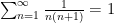
I’ve just uploaded to the arXiv my preprint “Perfectly packing a square by squares of nearly harmonic sidelength“. This paper concerns a variant of an old problem of Meir and Moser, who asks whether it is possible to perfectly pack squares of sidelength ${1/n}$ for ${n \geq 2}$ into a single square or rectangle of area ${\sum_{n=2}^\infty \frac{1}{n^2} = \frac{\pi^2}{6} - 1}$ . (The following variant problem, also posed by Meir and Moser and discussed for instance in this MathOverflow post, is perhaps even more well known: is it possible to perfectly pack rectangles of dimensions ${1/n \times 1/(n+1)}$ for ${n \geq 1}$ into a single square of area ${\sum_{n=1}^\infty \frac{1}{n(n+1)} = 1}$ ?) For the purposes of this paper, rectangles and squares are understood to have sides parallel to the axes, and a packing is perfect if it partitions the region being packed up to sets of measure zero. As one partial result towards these problems, it was shown by Paulhus that squares of sidelength ${1/n}$ for ${n \geq 2}$ can be packed (not quite perfectly) into a single rectangle of area ${\frac{\pi^2}{6} - 1 + \frac{1}{1244918662}}$ , and rectangles of dimensions ${1/n \times 1/n+1}$ for ${n \geq 1}$ can be packed (again not quite perfectly) into a single square of area ${1 + \frac{1}{10^9+1}}$ . (Paulhus’s paper had some gaps in it, but these were subsequently repaired by Grzegorek and Januszewski.)

Another direction in which partial progress has been made is to consider instead the problem of packing squares of sidelength ${n^{-t}}$ , ${n \geq 1}$ perfectly into a square or rectangle of total area ${\sum_{n=1}^\infty \frac{1}{n^{2t}}}$ , for some fixed constant ${t > 1/2}$ (this lower bound is needed to make the total area ${\sum_{n=1}^\infty \frac{1}{n^{2t}}}$ finite), with the aim being to get ${t}$ as close to ${1}$ as possible. Prior to this paper, the most recent advance in this direction was by Januszewski and Zielonka last year, who achieved such a packing in the range ${1/2 < t \leq 2/3}$ .

In this paper we are able to get ${t}$ arbitrarily close to ${1}$ (which turns out to be a “critical” value of this parameter), but at the expense of deleting the first few tiles:

Theorem 1 If ${1/2 < t < 1}$ , and ${n_0}$ is sufficiently large depending on ${t}$ , then one can pack squares of sidelength ${n^{-t}}$ , ${n \geq n_0}$ perfectly into a square of area ${\sum_{n=n_0}^\infty \frac{1}{n^{2t}}}$ .

As in previous works, the general strategy is to execute a greedy algorithm, which can be described somewhat incompletely as follows.

Step 1: Suppose that one has already managed to perfectly pack a square ${S}$ of area ${\sum_{n=n_0}^\infty \frac{1}{n^{2t}}}$ by squares of sidelength ${n^{-t}}$ for ${n_0 \leq n < n_1}$ , together with a further finite collection ${{\mathcal R}}$ of rectangles with disjoint interiors. (Initially, we would have ${n_1=n_0}$ and ${{\mathcal R} = \{S\}}$ , but these parameter will change over the course of the algorithm.)
Step 2: Amongst all the rectangles in ${{\mathcal R}}$ , locate the rectangle ${R}$ of the largest width (defined as the shorter of the two sidelengths of ${R}$ ).
Step 3: Pack (as efficiently as one can) squares of sidelength ${n^{-t}}$ for ${n_1 \leq n < n_2}$ into ${R}$ for some ${n_2>n_1}$ , and decompose the portion of ${R}$ not covered by this packing into rectangles ${{\mathcal R}'}$ .
Step 4: Replace ${n_1}$ by ${n_2}$ , replace ${{\mathcal R}}$ by ${({\mathcal R} \backslash \{R\}) \cup {\mathcal R}'}$ , and return to Step 1.

The main innovation of this paper is to perform Step 3 somewhat more efficiently than in previous papers.

The above algorithm can get stuck if one reaches a point where one has already packed squares of sidelength ${1/n^t}$ for ${n_0 \leq n < n_1}$ , but that all remaining rectangles ${R}$ in ${{\mathcal R}}$ have width less than ${n_1^{-t}}$ , in which case there is no obvious way to fit in the next square. If we let ${w(R)}$ and ${h(R)}$ denote the width and height of these rectangles ${R}$ , then the total area of the rectangles must be

$\displaystyle \sum_{R \in {\mathcal R}} w(R) h(R) = \sum_{n=n_0}^\infty \frac{1}{n^{2t}} - \sum_{n=n_0}^{n_1-1} \frac{1}{n^{2t}} \asymp n_1^{1-2t}$

and the total perimeter ${\mathrm{perim}({\mathcal R})}$ of these rectangles is

$\displaystyle \mathrm{perim}({\mathcal R}) = \sum_{R \in {\mathcal R}} 2(w(R)+h(R)) \asymp \sum_{R \in {\mathcal R}} h(R).$

Thus we have

$\displaystyle n_1^{1-2t} \ll \mathrm{perim}({\mathcal R}) \sup_{R \in {\mathcal R}} w(R)$

and so to ensure that there is at least one rectangle ${R}$ with ${w(R) \geq n_1^{-t}}$ it would be enough to have the perimeter bound

$\displaystyle \mathrm{perim}({\mathcal R}) \leq c n_1^{1-t}$

for a sufficiently small constant ${c>0}$ . It is here that we now see the critical nature of the exponent ${t=1}$ : for ${t<1}$ , the amount of perimeter we are permitted to have in the remaining rectangles increases as one progresses with the packing, but for ${t=1}$ the amount of perimeter one is “budgeted” for stays constant (and for ${t>1}$ the situation is even worse, in that the remaining rectangles ${{\mathcal R}}$ should steadily decrease in total perimeter).

In comparison, the perimeter of the squares that one has already packed is equal to

$\displaystyle \sum_{n=n_0}^{n_1-1} 4 n^{-t}$

which is comparable to ${n_1^{1-t}}$ for ${n_1}$ large (with the constants blowing up as ${t}$ approaches the critical value of ${1}$ ). In previous algorithms, the total perimeter of the remainder rectangles ${{\mathcal R}}$ was basically comparable to the perimeter of the squares already packed, and this is the main reason why the results only worked when ${t}$ was sufficiently far away from ${1}$ . In my paper, I am able to get the perimeter of ${{\mathcal R}}$ significantly smaller than the perimeter of the squares already packed, by grouping those squares into lattice-like clusters (of about ${M^2}$ squares arranged in an ${M \times M}$ pattern), and sliding the squares in each cluster together to almost entirely eliminate the wasted space between each square, leaving only the space around the cluster as the main source of residual perimeter, which will be comparable to about ${M n_1^{-t}}$ per cluster, as compared to the total perimeter of the squares in the cluster which is comparable to ${M^2 n_1^{-t}}$ . This strategy is perhaps easiest to illustrate with a picture, in which ${3 \times 4}$ squares ${S_{i,j}}$ of slowly decreasing sidelength are packed together with relatively little wasted space:

By choosing the parameter ${M}$ suitably large (and taking ${n_0}$ sufficiently large depending on ${M}$ ), one can then prove the theorem. (In order to do some technical bookkeeping and to allow one to close an induction in the verification of the algorithm’s correctness, it is convenient to replace the perimeter ${\sum_{R \in {\mathcal R}} 2(w(R)+h(R))}$ by a slightly weighted variant ${\sum_{R \in {\mathcal R}} w(R)^\delta h(R)}$ for a small exponent ${\delta}$ , but this is a somewhat artificial device that somewhat obscures the main ideas.)

The spherical Cayley-Menger determinant and the radius of the Earth

25 May, 2019 in expository, math.GM, math.MG | Tags: Geodesy, recreational mathematics, spherical geometry | by Terence Tao | 28 comments

Given three points ${A,B,C}$ in the plane, the distances ${|AB|, |BC|, |AC|}$ between them have to be non-negative and obey the triangle inequalities

$\displaystyle |AB| \leq |BC| + |AC|, |BC| \leq |AC| + |AB|, |AC| \leq |AB| + |BC|$

but are otherwise unconstrained. But if one has four points ${A,B,C,D}$ in the plane, then there is an additional constraint connecting the six distances ${|AB|, |AC|, |AD|, |BC|, |BD|, |CD|}$ between them, coming from the Cayley-Menger determinant:

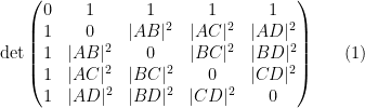
Proposition 1 (Cayley-Menger determinant) If ${A,B,C,D}$ are four points in the plane, then the Cayley-Menger determinant

$\displaystyle \mathrm{det} \begin{pmatrix} 0 & 1 & 1 & 1 & 1 \\ 1 & 0 & |AB|^2 & |AC|^2 & |AD|^2 \\ 1 & |AB|^2 & 0 & |BC|^2 & |BD|^2 \\ 1 & |AC|^2 & |BC|^2 & 0 & |CD|^2 \\ 1 & |AD|^2 & |BD|^2 & |CD|^2 & 0 \end{pmatrix} \ \ \ \ \ (1)$

vanishes.

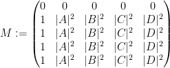
Proof: If we view ${A,B,C,D}$ as vectors in ${{\bf R}^2}$ , then we have the usual cosine rule ${|AB|^2 = |A|^2 + |B|^2 - 2 A \cdot B}$ , and similarly for all the other distances. The ${5 \times 5}$ matrix appearing in (1) can then be written as ${M+M^T-2\tilde G}$ , where ${M}$ is the matrix

$\displaystyle M := \begin{pmatrix} 0 & 0 & 0 & 0 & 0 \\ 1 & |A|^2 & |B|^2 & |C|^2 & |D|^2 \\ 1 & |A|^2 & |B|^2 & |C|^2 & |D|^2 \\ 1 & |A|^2 & |B|^2 & |C|^2 & |D|^2 \\ 1 & |A|^2 & |B|^2 & |C|^2 & |D|^2 \end{pmatrix}$

and ${\tilde G}$ is the (augmented) Gram matrix

$\displaystyle \tilde G := \begin{pmatrix} 0 & 0 & 0 & 0 & 0 \\ 0 & A \cdot A & A \cdot B & A \cdot C & A \cdot D \\ 0 & B \cdot A & B \cdot B & B \cdot C & B \cdot D \\ 0 & C \cdot A & C \cdot B & C \cdot C & C \cdot D \\ 0 & D \cdot A & D \cdot B & D \cdot C & D \cdot D \end{pmatrix}.$

The matrix ${M}$ is a rank one matrix, and so ${M^T}$ is also. The Gram matrix ${\tilde G}$ factorises as ${\tilde G = \tilde \Sigma \tilde \Sigma^T}$ , where ${\tilde \Sigma}$ is the ${5 \times 2}$ matrix with rows ${0,A,B,C,D}$ , and thus has rank at most ${2}$ . Therefore the matrix ${M+M^T-2\tilde G}$ in (1) has rank at most ${1+1+2=4}$ , and hence has determinant zero as claimed. $\Box$

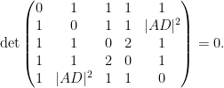
For instance, if we know that ${|AB|=|AC|=|DB|=|DC|=1}$ and ${|BC|=\sqrt{2}}$ , then in order for ${A,B,C,D}$ to be coplanar, the remaining distance ${|AD|}$ has to obey the equation

$\displaystyle \mathrm{det} \begin{pmatrix} 0 & 1 & 1 & 1 & 1 \\ 1 & 0 & 1 & 1 & |AD|^2 \\ 1 & 1 & 0 & 2 & 1 \\ 1 & 1 & 2 & 0 & 1 \\ 1 & |AD|^2 & 1 & 1 & 0 \end{pmatrix} = 0.$

After some calculation the left-hand side simplifies to ${-4 |AD|^4 + 8 |AD|^2}$ , so the non-negative quantity is constrained to equal either ${0}$ or ${\sqrt{2}}$ . The former happens when ${A,B,C}$ form a unit right-angled triangle with right angle at ${A}$ and ${D=A}$ ; the latter happens when ${A,B,D,C}$ form the vertices of a unit square traversed in that order. Any other value for ${|AD|}$ is not compatible with the hypothesis for ${A,B,C,D}$ lying on a plane; hence the Cayley-Menger determinant can be used as a test for planarity.

Now suppose that we have four points ${A,B,C,D}$ on a sphere ${S_R}$ of radius ${R}$ , with six distances ${|AB|_R, |AC|_R, |AD|_R, |BC|_R, |BD|_R, |AD|_R}$ now measured as lengths of arcs on the sphere. There is a spherical analogue of the Cayley-Menger determinant:

Proposition 2 (Spherical Cayley-Menger determinant) If ${A,B,C,D}$ are four points on a sphere ${S_R}$ of radius ${R}$ in ${{\bf R}^3}$ , then the spherical Cayley-Menger determinant

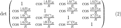
$\displaystyle \mathrm{det} \begin{pmatrix} 1 & \cos \frac{|AB|_R}{R} & \cos \frac{|AC|_R}{R} & \cos \frac{|AD|_R}{R} \\ \cos \frac{|AB|_R}{R} & 1 & \cos \frac{|BC|_R}{R} & \cos \frac{|BD|_R}{R} \\ \cos \frac{|AC|_R}{R} & \cos \frac{|BC|_R}{R} & 1 & \cos \frac{|CD|_R}{R} \\ \cos \frac{|AD|_R}{R} & \cos \frac{|BD|_R}{R} & \cos \frac{|CD|_R}{R} & 1 \end{pmatrix} \ \ \ \ \ (2)$

vanishes.

Proof: We can assume that the sphere ${S_R}$ is centred at the origin of ${{\bf R}^3}$ , and view ${A,B,C,D}$ as vectors in ${{\bf R}^3}$ of magnitude ${R}$ . The angle subtended by ${AB}$ from the origin is ${|AB|_R/R}$ , so by the cosine rule we have

$\displaystyle A \cdot B = R^{2} \cos \frac{|AB|_R}{R}.$

Similarly for all the other inner products. Thus the matrix in (2) can be written as ${R^{-2} G}$ , where ${G}$ is the Gram matrix

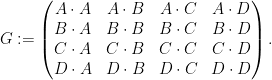
$\displaystyle G := \begin{pmatrix} A \cdot A & A \cdot B & A \cdot C & A \cdot D \\ B \cdot A & B \cdot B & B \cdot C & B \cdot D \\ C \cdot A & C \cdot B & C \cdot C & C \cdot D \\ D \cdot A & D \cdot B & D \cdot C & D \cdot D \end{pmatrix}.$

We can factor ${G = \Sigma \Sigma^T}$ where ${\Sigma}$ is the ${4 \times 3}$ matrix with rows ${A,B,C,D}$ . Thus ${R^{-2} G}$ has rank at most ${3}$ and thus the determinant vanishes as required. $\Box$

Just as the Cayley-Menger determinant can be used to test for coplanarity, the spherical Cayley-Menger determinant can be used to test for lying on a sphere of radius ${R}$ . For instance, if we know that ${A,B,C,D}$ lie on ${S_R}$ and ${|AB|_R, |AC|_R, |BC|_R, |BD|_R, |CD|_R}$ are all equal to ${\pi R/2}$ , then the above proposition gives

$\displaystyle \mathrm{det} \begin{pmatrix} 1 & 0 & 0 & \cos \frac{|AD|_R}{R} \\ 0 & 1 & 0 & 0 \\ 0 & 0 & 1 & 0 \\ \cos \frac{|AD|_R}{R} & 0 & 0 & 1 \end{pmatrix} = 0.$

The left-hand side evaluates to ${1 - \cos^2 \frac{|AD|_R}{R}}$ ; as ${|AD|_R}$ lies between ${0}$ and ${\pi R}$ , the only choices for this distance are then ${0}$ and ${\pi R}$ . The former happens for instance when ${A}$ lies on the north pole ${(R,0,0)}$ , ${B = (0,R,0), C = (0,R,0)}$ are points on the equator with longitudes differing by 90 degrees, and ${D=(R,0,0)}$ is also equal to the north pole; the latter occurs when ${D=(-R,0,0)}$ is instead placed on the south pole.

The Cayley-Menger and spherical Cayley-Menger determinants look slightly different from each other, but one can transform the latter into something resembling the former by row and column operations. Indeed, the determinant (2) can be rewritten as

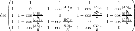
$\displaystyle \mathrm{det} \begin{pmatrix} 1 & 1 & 1 & 1 & 1 \\ 1 & 0 & 1 - \cos \frac{|AB|_R}{R} & 1 - \cos \frac{|AC|_R}{R} & 1 - \cos \frac{|AD|_R}{R} \\ 1 & 1-\cos \frac{|AB|_R}{R} & 0 & 1-\cos \frac{|BC|_R}{R} & 1- \cos \frac{|BD|_R}{R} \\ 1 & 1-\cos \frac{|AC|_R}{R} & 1-\cos \frac{|BC|_R}{R} & 0 & 1-\cos \frac{|CD|_R}{R} \\ 1 & 1-\cos \frac{|AD|_R}{R} & 1-\cos \frac{|BD|_R}{R} & 1- \cos \frac{|CD|_R}{R} & 0 \end{pmatrix}$

and by further row and column operations, this determinant vanishes if and only if the determinant

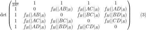
$\displaystyle \mathrm{det} \begin{pmatrix} \frac{1}{2R^2} & 1 & 1 & 1 & 1 \\ 1 & 0 & f_R(|AB|_R) & f_R(|AC|_R) & f_R(|AD|_R) \\ 1 & f_R(|AB|_R) & 0 & f_R(|BC|_R) & f_R(|BD|_R) \\ 1 & f_R(|AC|_R) & f_R(|BC|_R) & 0 & f_R(|CD|_R) \\ 1 & f_R(|AD|_R) & f_R(|BD|_R) & f_R(|CD|_R) & 0 \end{pmatrix} \ \ \ \ \ (3)$

vanishes, where ${f_R(x) := 2R^2 (1-\cos \frac{x}{R})}$ . In the limit ${R \rightarrow \infty}$ (so that the curvature of the sphere ${S_R}$ tends to zero), ${|AB|_R}$ tends to ${|AB|}$ , and by Taylor expansion ${f_R(|AB|_R)}$ tends to ${|AB|^2}$ ; similarly for the other distances. Now we see that the planar Cayley-Menger determinant emerges as the limit of (3) as ${R \rightarrow \infty}$ , as would be expected from the intuition that a plane is essentially a sphere of infinite radius.

In principle, one can now estimate the radius ${R}$ of the Earth (assuming that it is either a sphere ${S_R}$ or a flat plane ${S_\infty}$ ) if one is given the six distances ${|AB|_R, |AC|_R, |AD|_R, |BC|_R, |BD|_R, |CD|_R}$ between four points ${A,B,C,D}$ on the Earth. Of course, if one wishes to do so, one should have ${A,B,C,D}$ rather far apart from each other, since otherwise it would be difficult to for instance distinguish the round Earth from a flat one. As an experiment, and just for fun, I wanted to see how accurate this would be with some real world data. I decided to take ${A}$ , ${B}$ , ${C}$ , ${D}$ be the cities of London, Los Angeles, Tokyo, and Dubai respectively. As an initial test, I used distances from this online flight calculator, measured in kilometers:

$\displaystyle |AB|_R = 8790$

$\displaystyle |AC|_R = 9597 \mathrm{km}$

$\displaystyle |AD|_R = 5488\mathrm{km}$

$\displaystyle |BC|_R = 8849\mathrm{km}$

$\displaystyle |BD|_R = 13435\mathrm{km}$

$\displaystyle |CD|_R = 7957\mathrm{km}.$

Given that the true radius of the earth was about ${R_0 := 6371 \mathrm{km}}$ kilometers, I chose the change of variables ${R = R_0/k}$ (so that ${k=1}$ corresponds to the round Earth model with the commonly accepted value for the Earth’s radius, and ${k=0}$ corresponds to the flat Earth), and obtained the following plot for (3):

In particular, the determinant does indeed come very close to vanishing when ${k=1}$ , which is unsurprising since, as explained on the web site, the online flight calculator uses a model in which the Earth is an ellipsoid of radii close to ${6371}$ km. There is another radius that would also be compatible with this data at ${k\approx 1.3}$ (corresponding to an Earth of radius about ${4900}$ km), but presumably one could rule out this as a spurious coincidence by experimenting with other quadruples of cities than the ones I selected. On the other hand, these distances are highly incompatible with the flat Earth model ${k=0}$ ; one could also see this with a piece of paper and a ruler by trying to lay down four points ${A,B,C,D}$ on the paper with (an appropriately rescaled) version of the above distances (e.g., with ${|AB| = 8.790 \mathrm{cm}}$ , ${|AC| = 9.597 \mathrm{cm}}$ , etc.).

If instead one goes to the flight time calculator and uses flight travel times instead of distances, one now gets the following data (measured in hours):

$\displaystyle |AB|_R = 10\mathrm{h}\ 3\mathrm{m}$

$\displaystyle |AC|_R = 11\mathrm{h}\ 49\mathrm{m}$

$\displaystyle |AD|_R = 6\mathrm{h}\ 56\mathrm{m}$

$\displaystyle |BC|_R = 10\mathrm{h}\ 56\mathrm{m}$

$\displaystyle |BD|_R = 16\mathrm{h}\ 23\mathrm{m}$

$\displaystyle |CD|_R = 9\mathrm{h}\ 52\mathrm{m}.$

Assuming that planes travel at about ${800}$ kilometers per hour, the true radius of the Earth should be about ${R_1 := 8\mathrm{h}}$ of flight time. If one then uses the normalisation ${R = R_1/k}$ , one obtains the following plot:

Not too surprisingly, this is basically a rescaled version of the previous plot, with vanishing near ${k=1}$ and at ${k=1.3}$ . (The website for the flight calculator does say it calculates short and long haul flight times slightly differently, which may be the cause of the slight discrepancies between this figure and the previous one.)

Of course, these two data sets are “cheating” since they come from a model which already presupposes what the radius of the Earth is. But one can input real world flight times between these four cities instead of the above idealised data. Here one runs into the issue that the flight time from ${A}$ to ${B}$ is not necessarily the same as that from ${B}$ to ${A}$ due to such factors as windspeed. For instance, I looked up the online flight time from Tokyo to Dubai to be 11 hours and 10 minutes, whereas the online flight time from Dubai to Tokyo was 9 hours and 50 minutes. The simplest thing to do here is take an arithmetic mean of the two times as a preliminary estimate for the flight time without windspeed factors, thus for instance the Tokyo-Dubai flight time would now be 10 hours and 30 minutes, and more generally

$\displaystyle |AB|_R = 10\mathrm{h}\ 47\mathrm{m}$

$\displaystyle |AC|_R = 12\mathrm{h}\ 0\mathrm{m}$

$\displaystyle |AD|_R = 7\mathrm{h}\ 17\mathrm{m}$

$\displaystyle |BC|_R = 10\mathrm{h}\ 50\mathrm{m}$

$\displaystyle |BD|_R = 15\mathrm{h}\ 55\mathrm{m}$

$\displaystyle |CD|_R = 10\mathrm{h}\ 30\mathrm{m}.$

This data is not too far off from the online calculator data, but it does distort the graph slightly (taking ${R=8/k}$ as before):

Now one gets estimates for the radius of the Earth that are off by about a factor of ${2}$ from the truth, although the ${k=1}$ round Earth model still is twice as accurate as the flat Earth model ${k=0}$ .

Given that windspeed should additively affect flight velocity rather than flight time, and the two are inversely proportional to each other, it is more natural to take a harmonic mean rather than an arithmetic mean. This gives the slightly different values

$\displaystyle |AB|_R = 10\mathrm{h}\ 51\mathrm{m}$

$\displaystyle |AC|_R = 11\mathrm{h}\ 59\mathrm{m}$

$\displaystyle |AD|_R = 7\mathrm{h}\ 16\mathrm{m}$

$\displaystyle |BC|_R = 10\mathrm{h}\ 46\mathrm{m}$

$\displaystyle |BD|_R = 15\mathrm{h}\ 54\mathrm{m}$

$\displaystyle |CD|_R = 10\mathrm{h}\ 27\mathrm{m}$

but one still gets essentially the same plot:

So the inaccuracies are presumably coming from some other source. (Note for instance that the true flight time from Tokyo to Dubai is about ${6\%}$ greater than the calculator predicts, while the flight time from LA to Dubai is about ${3\%}$ less; these sorts of errors seem to pile up in this calculation.) Nevertheless, it does seem that flight time data is (barely) enough to establish the roundness of the Earth and obtain a somewhat ballpark estimate for its radius. (I assume that the fit would be better if one could include some Southern Hemisphere cities such as Sydney or Santiago, but I was not able to find a good quadruple of widely spaced cities on both hemispheres for which there were direct flights between all six pairs.)

Embedding the Heisenberg group into a bounded dimensional Euclidean space with optimal distortion

26 November, 2018 in math.AP, math.MG, paper | Tags: bilipschitz embedding, Heisenberg group, Nash embedding theorem | by Terence Tao | 13 comments

I’ve just uploaded to the arXiv my paper “Embedding the Heisenberg group into a bounded dimensional Euclidean space with optimal distortion“, submitted to Revista Matematica Iberoamericana. This paper concerns the extent to which one can accurately embed the metric structure of the Heisenberg group

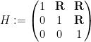
$\displaystyle H := \begin{pmatrix} 1 & {\bf R} & {\bf R} \\ 0 & 1 & {\bf R} \\ 0 & 0 & 1 \end{pmatrix}$

into Euclidean space, which we can write as ${\{ [x,y,z]: x,y,z \in {\bf R} \}}$ with the notation

$\displaystyle [x,y,z] := \begin{pmatrix} 1 & x & z \\ 0 & 1 & y \\ 0 & 0 & 1 \end{pmatrix}.$

Here we give ${H}$ the right-invariant Carnot-Carathéodory metric ${d}$ coming from the right-invariant vector fields

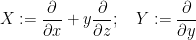
$\displaystyle X := \frac{\partial}{\partial x} + y \frac{\partial}{\partial z}; \quad Y := \frac{\partial}{\partial y}$

but not from the commutator vector field

$\displaystyle Z := [Y,X] = \frac{\partial}{\partial z}.$

This gives ${H}$ the geometry of a Carnot group. As observed by Semmes, it follows from the Carnot group differentiation theory of Pansu that there is no bilipschitz map from ${(H,d)}$ to any Euclidean space ${{\bf R}^D}$ or even to ${\ell^2}$ , since such a map must be differentiable almost everywhere in the sense of Carnot groups, which in particular shows that the derivative map annihilate ${Z}$ almost everywhere, which is incompatible with being bilipschitz.

On the other hand, if one snowflakes the Heisenberg group by replacing the metric ${d}$ with ${d^{1-\varepsilon}}$ for some ${0 < \varepsilon < 1}$ , then it follows from the general theory of Assouad on embedding snowflaked metrics of doubling spaces that ${(H,d^{1-\varepsilon})}$ may be embedded in a bilipschitz fashion into ${\ell^2}$ , or even to ${{\bf R}^{D_\varepsilon}}$ for some ${D_\varepsilon}$ depending on ${\varepsilon}$ .

Of course, the distortion of this bilipschitz embedding must degenerate in the limit ${\varepsilon \rightarrow 0}$ . From the work of Austin-Naor-Tessera and Naor-Neiman it follows that ${(H,d^{1-\varepsilon})}$ may be embedded into ${\ell^2}$ with a distortion of ${O( \varepsilon^{-1/2} )}$ , but no better. The Naor-Neiman paper also embeds ${(H,d^{1-\varepsilon})}$ into a finite-dimensional space ${{\bf R}^D}$ with ${D}$ independent of ${\varepsilon}$ , but at the cost of worsening the distortion to ${O(\varepsilon^{-1})}$ . They then posed the question of whether this worsening of the distortion is necessary.

The main result of this paper answers this question in the negative:

Theorem 1 There exists an absolute constant ${D}$ such that ${(H,d^{1-\varepsilon})}$ may be embedded into ${{\bf R}^D}$ in a bilipschitz fashion with distortion ${O(\varepsilon^{-1/2})}$ for any ${0 < \varepsilon \leq 1/2}$ .

To motivate the proof of this theorem, let us first present a bilipschitz map ${\Phi: {\bf R} \rightarrow \ell^2}$ from the snowflaked line ${({\bf R},d_{\bf R}^{1-\varepsilon})}$ (with ${d_{\bf R}}$ being the usual metric on ${{\bf R}}$ ) into complex Hilbert space ${\ell^2({\bf C})}$ . The map is given explicitly as a Weierstrass type function

$\displaystyle \Phi(x) := \sum_{k \in {\bf Z}} 2^{-\varepsilon k} (\phi_k(x) - \phi_k(0))$

where for each ${k}$ , ${\phi_k: {\bf R} \rightarrow \ell^2}$ is the function

$\displaystyle \phi_k(x) := 2^k e^{2\pi i x / 2^k} e_k.$

and ${(e_k)_{k \in {\bf Z}}}$ are an orthonormal basis for ${\ell^2({\bf C})}$ . The subtracting of the constant ${\phi_k(0)}$ is purely in order to make the sum convergent as ${k \rightarrow \infty}$ . If ${x,y \in {\bf R}}$ are such that ${2^{k_0-2} \leq d_{\bf R}(x,y) \leq 2^{k_0-1}}$ for some integer ${k_0}$ , one can easily check the bounds

$\displaystyle 2^{-\varepsilon k}|\phi_k(x) - \phi_k(y)| \lesssim d_{\bf R}(x,y)^{(1-\varepsilon)} \min( 2^{-(1-\varepsilon) (k_0-k)}, 2^{-\varepsilon (k-k_0)} )$

with the lower bound

$\displaystyle 2^{-\varepsilon k_0}|\phi_{k_0}(x) - \phi_{k_0}(y)| \gtrsim d_{\bf R}(x,y)^{(1-\varepsilon)}$

at which point one finds that

$\displaystyle d_{\bf R}(x,y)^{1-\varepsilon} \lesssim |\Phi(x) - \Phi(y)| \lesssim \varepsilon^{-1/2} d_{\bf R}(x,y)^{1-\varepsilon}$

as desired.

The key here was that each function ${\phi_k}$ oscillated at a different spatial scale ${2^k}$ , and the functions were all orthogonal to each other (so that the upper bound involved a factor of ${\varepsilon^{-1/2}}$ rather than ${\varepsilon^{-1}}$ ). One can replicate this example for the Heisenberg group without much difficulty. Indeed, if we let ${\Gamma := \{ [a,b,c]: a,b,c \in {\bf Z} \}}$ be the discrete Heisenberg group, then the nilmanifold ${H/\Gamma}$ is a three-dimensional smooth compact manifold; thus, by the Whitney embedding theorem, it smoothly embeds into ${{\bf R}^6}$ . This gives a smooth immersion ${\phi: H \rightarrow {\bf R}^6}$ which is ${\Gamma}$ -automorphic in the sense that ${\phi(p\gamma) = \phi(p)}$ for all ${p \in H}$ and ${\gamma \in \Gamma}$ . If one then defines ${\phi_k: H \rightarrow \ell^2 \otimes {\bf R}^6}$ to be the function

$\displaystyle \phi_k(p) := 2^k \phi( \delta_{2^{-k}}(p) ) \otimes e_k$

where ${\delta_\lambda: H \rightarrow H}$ is the scaling map

$\displaystyle \delta_\lambda([x,y,z]) := [\lambda x, \lambda y, \lambda^2 z],$

then one can repeat the previous arguments to obtain the required bilipschitz bounds

$\displaystyle d(p,q)^{1-\varepsilon} \lesssim |\Phi(p) - \Phi(q) \lesssim \varepsilon^{-1/2} d(p,q)^{1-\varepsilon}$

for the function

$\displaystyle \Phi(p) :=\sum_{k \in {\bf Z}} 2^{-\varepsilon k} (\phi_k(p) - \phi_k(0)).$

To adapt this construction to bounded dimension, the main obstruction was the requirement that the ${\phi_k}$ took values in orthogonal subspaces. But if one works things out carefully, it is enough to require the weaker orthogonality requirement

$\displaystyle B( \phi_{k_0}, \sum_{k>k_0} 2^{-\varepsilon(k-k_0)} \phi_k ) = 0$

for all ${k_0 \in {\bf Z}}$ , where ${B(\phi, \psi): H \rightarrow {\bf R}^2}$ is the bilinear form

$\displaystyle B(\phi,\psi) := (X \phi \cdot X \psi, Y \phi \cdot Y \psi ).$

One can then try to construct the ${\phi_k: H \rightarrow {\bf R}^D}$ for bounded dimension ${D}$ by an iterative argument. After some standard reductions, the problem becomes this (roughly speaking): given a smooth, slowly varying function ${\psi: H \rightarrow {\bf R}^{D}}$ whose derivatives obey certain quantitative upper and lower bounds, construct a smooth oscillating function ${\phi: H \rightarrow {\bf R}^{D}}$ , whose derivatives also obey certain quantitative upper and lower bounds, which obey the equation

$\displaystyle B(\phi,\psi) = 0. \ \ \ \ \ (1)$

We view this as an underdetermined system of differential equations for ${\phi}$ (two equations in ${D}$ unknowns; after some reductions, our ${D}$ can be taken to be the explicit value ${36}$ ). The trivial solution ${\phi=0}$ to this equation will be inadmissible for our purposes due to the lower bounds we will require on ${\phi}$ (in order to obtain the quantitative immersion property mentioned previously, as well as for a stronger “freeness” property that is needed to close the iteration). Because this construction will need to be iterated, it will be essential that the regularity control on ${\phi}$ is the same as that on ${\psi}$ ; one cannot afford to “lose derivatives” when passing from ${\psi}$ to ${\phi}$ .

This problem has some formal similarities with the isometric embedding problem (discussed for instance in this previous post), which can be viewed as the problem of solving an equation of the form ${Q(\phi,\phi) = g}$ , where ${(M,g)}$ is a Riemannian manifold and ${Q}$ is the bilinear form

$\displaystyle Q(\phi,\psi)_{ij} = \partial_i \phi \cdot \partial_j \psi.$

The isometric embedding problem also has the key obstacle that naive attempts to solve the equation ${Q(\phi,\phi)=g}$ iteratively can lead to an undesirable “loss of derivatives” that prevents one from iterating indefinitely. This obstacle was famously resolved by the Nash-Moser iteration scheme in which one alternates between perturbatively adjusting an approximate solution to improve the residual error term, and mollifying the resulting perturbation to counteract the loss of derivatives. The current equation (1) differs in some key respects from the isometric embedding equation ${Q(\phi,\phi)=g}$ , in particular being linear in the unknown field ${\phi}$ rather than quadratic; nevertheless the key obstacle is the same, namely that naive attempts to solve either equation lose derivatives. Our approach to solving (1) was inspired by the Nash-Moser scheme; in retrospect, I also found similarities with Uchiyama’s constructive proof of the Fefferman-Stein decomposition theorem, discussed in this previous post (and in this recent one).

To motivate this iteration, we first express ${B(\phi,\psi)}$ using the product rule in a form that does not place derivatives directly on the unknown ${\phi}$ :

$\displaystyle B(\phi,\psi) = \left( W(\phi \cdot W \psi) - \phi \cdot WW \psi\right)_{W = X,Y} \ \ \ \ \ (2)$

This reveals that one can construct solutions ${\phi}$ to (1) by solving the system of equations

$\displaystyle \phi \cdot W \psi = \phi \cdot WW \psi = 0 \ \ \ \ \ (3)$

for ${W \in \{X, Y \}}$ . Because this system is zeroth order in ${\phi}$ , this can easily be done by linear algebra (even in the presence of a forcing term ${B(\phi,\psi)=F}$ ) if one imposes a “freeness” condition (analogous to the notion of a free embedding in the isometric embedding problem) that ${X \psi(p), Y \psi(p), XX \psi(p), YY \psi(p)}$ are linearly independent at each point ${p}$ , which (together with some other technical conditions of a similar nature) one then adds to the list of upper and lower bounds required on ${\psi}$ (with a related bound then imposed on ${\phi}$ , in order to close the iteration). However, as mentioned previously, there is a “loss of derivatives” problem with this construction: due to the presence of the differential operators ${W}$ in (3), a solution ${\phi}$ constructed by this method can only be expected to have two degrees less regularity than ${\psi}$ at best, which makes this construction unsuitable for iteration.

To get around this obstacle (which also prominently appears when solving (linearisations of) the isometric embedding equation ${Q(\phi,\phi)=g}$ ), we instead first construct a smooth, low-frequency solution ${\phi_{\leq N_0} \colon H \rightarrow {\bf R}^{D}}$ to a low-frequency equation

$\displaystyle B( \phi_{\leq N_0}, P_{\leq N_0} \psi ) = 0 \ \ \ \ \ (4)$

where ${P_{\leq N_0} \psi}$ is a mollification of ${\psi}$ (of Littlewood-Paley type) applied at a small spatial scale ${1/N_0}$ for some ${N_0}$ , and then gradually relax the frequency cutoff ${P_{\leq N_0}}$ to deform this low frequency solution ${\phi_{\leq N_0}}$ to a solution ${\phi}$ of the actual equation (1).

We will construct the low-frequency solution ${\phi_{\leq N_0}}$ rather explicitly, using the Whitney embedding theorem to construct an initial oscillating map ${f}$ into a very low dimensional space ${{\bf R}^6}$ , composing it with a Veronese type embedding into a slightly larger dimensional space ${{\bf R}^{27}}$ to obtain a required “freeness” property, and then composing further with a slowly varying isometry ${U(p) \colon {\bf R}^{27} \rightarrow {\bf R}^{36}}$ depending on ${P_{\leq N_0}}$ and constructed by a quantitative topological lemma (relying ultimately on the vanishing of the first few homotopy groups of high-dimensional spheres), in order to obtain the required orthogonality (4). (This sort of “quantitative null-homotopy” was first proposed by Gromov, with some recent progress on optimal bounds by Chambers-Manin-Weinberger and by Chambers-Dotterer-Manin-Weinberger, but we will not need these more advanced results here, as one can rely on the classical qualitative vanishing ${\pi^k(S^d)=0}$ for ${k < d}$ together with a compactness argument to obtain (ineffective) quantitative bounds, which suffice for this application).

To perform the deformation of ${\phi_{\leq N_0}}$ into ${\phi}$ , we must solve what is essentially the linearised equation

$\displaystyle B( \dot \phi, \psi ) + B( \phi, \dot \psi ) = 0 \ \ \ \ \ (5)$

of (1) when ${\phi}$ , ${\psi}$ (viewed as low frequency functions) are both being deformed at some rates ${\dot \phi, \dot \psi}$ (which should be viewed as high frequency functions). To avoid losing derivatives, the magnitude of the deformation ${\dot \phi}$ in ${\phi}$ should not be significantly greater than the magnitude of the deformation ${\dot \psi}$ in ${\psi}$ , when measured in the same function space norms.

As before, if one directly solves the difference equation (5) using a naive application of (2) with ${B(\phi,\dot \psi)}$ treated as a forcing term, one will lose at least one derivative of regularity when passing from ${\dot \psi}$ to ${\dot \phi}$ . However, observe that (2) (and the symmetry ${B(\phi, \dot \psi) = B(\dot \psi,\phi)}$ ) can be used to obtain the identity

$\displaystyle B( \dot \phi, \psi ) + B( \phi, \dot \psi ) = \left( W(\dot \phi \cdot W \psi + \dot \psi \cdot W \phi) - (\dot \phi \cdot WW \psi + \dot \psi \cdot WW \phi)\right)_{W = X,Y} \ \ \ \ \ (6)$

and then one can solve (5) by solving the system of equations

$\displaystyle \dot \phi \cdot W \psi = - \dot \psi \cdot W \phi$

for ${W \in \{X,XX,Y,YY\}}$ . The key point here is that this system is zeroth order in both ${\dot \phi}$ and ${\dot \psi}$ , so one can solve this system without losing any derivatives when passing from ${\dot \psi}$ to ${\dot \phi}$ ; compare this situation with that of the superficially similar system

$\displaystyle \dot \phi \cdot W \psi = - \phi \cdot W \dot \psi$

that one would obtain from naively linearising (3) without exploiting the symmetry of ${B}$ . There is still however one residual “loss of derivatives” problem arising from the presence of a differential operator ${W}$ on the ${\phi}$ term, which prevents one from directly evolving this iteration scheme in time without losing regularity in ${\phi}$ . It is here that we borrow the final key idea of the Nash-Moser scheme, which is to replace ${\phi}$ by a mollified version ${P_{\leq N} \phi}$ of itself (where the projection ${P_{\leq N}}$ depends on the time parameter). This creates an error term in (5), but it turns out that this error term is quite small and smooth (being a “high-high paraproduct” of ${\nabla \phi}$ and ${\nabla\psi}$ , it ends up being far more regular than either ${\phi}$ or ${\psi}$ , even with the presence of the derivatives) and can be iterated away provided that the initial frequency cutoff ${N_0}$ is large and the function ${\psi}$ has a fairly high (but finite) amount of regularity (we will eventually use the Hölder space ${C^{20,\alpha}}$ on the Heisenberg group to measure this).

246C notes 2: Circle packings, conformal maps, and quasiconformal maps

12 April, 2018 in 246C - complex analysis, math.CV, math.MG | Tags: circle packing, quasiconformal mapping, Riemann mapping theorem | by Terence Tao | 32 comments

Previous set of notes: Notes 1. Next set of notes: Notes 3.

We now leave the topic of Riemann surfaces, and turn now to the (loosely related) topic of conformal mapping (and quasiconformal mapping). Recall that a conformal map ${f: U \rightarrow V}$ from an open subset ${U}$ of the complex plane to another open set ${V}$ is a map that is holomorphic and bijective, which (by Rouché’s theorem) also forces the derivative of ${f}$ to be nowhere vanishing. We then say that the two open sets ${U,V}$ are conformally equivalent. From the Cauchy-Riemann equations we see that conformal maps are orientation-preserving and angle-preserving; from the Newton approximation ${f( z_0 + \Delta z) \approx f(z_0) + f'(z_0) \Delta z + O( |\Delta z|^2)}$ we see that they almost preserve small circles, indeed for ${\varepsilon}$ small the circle ${\{ z: |z-z_0| = \varepsilon\}}$ will approximately map to ${\{ w: |w - f(z_0)| = |f'(z_0)| \varepsilon \}}$ .

In previous quarters, we proved a fundamental theorem about this concept, the Riemann mapping theorem:

Theorem 1 (Riemann mapping theorem) Let ${U}$ be a simply connected open subset of ${{\bf C}}$ that is not all of ${{\bf C}}$ . Then ${U}$ is conformally equivalent to the unit disk ${D(0,1)}$ .

This theorem was proven in these 246A lecture notes, using an argument of Koebe. At a very high level, one can sketch Koebe’s proof of the Riemann mapping theorem as follows: among all the injective holomorphic maps ${f: U \rightarrow D(0,1)}$ from ${U}$ to ${D(0,1)}$ that map some fixed point ${z_0 \in U}$ to ${0}$ , pick one that maximises the magnitude ${|f'(z_0)|}$ of the derivative (ignoring for this discussion the issue of proving that a maximiser exists). If ${f(U)}$ avoids some point in ${D(0,1)}$ , one can compose ${f}$ with various holomorphic maps and use Schwarz’s lemma and the chain rule to increase ${|f'(z_0)|}$ without destroying injectivity; see the previous lecture notes for details. The conformal map ${\phi: U \rightarrow D(0,1)}$ is unique up to Möbius automorphisms of the disk; one can fix the map by picking two distinct points ${z_0,z_1}$ in ${U}$ , and requiring ${\phi(z_0)}$ to be zero and ${\phi(z_1)}$ to be positive real.

It is a beautiful observation of Thurston that the concept of a conformal mapping has a discrete counterpart, namely the mapping of one circle packing to another. Furthermore, one can run a version of Koebe’s argument (using now a discrete version of Perron’s method) to prove the Riemann mapping theorem through circle packings. In principle, this leads to a mostly elementary approach to conformal geometry, based on extremely classical mathematics that goes all the way back to Apollonius. However, in order to prove the basic existence and uniqueness theorems of circle packing, as well as the convergence to conformal maps in the continuous limit, it seems to be necessary (or at least highly convenient) to use much more modern machinery, including the theory of quasiconformal mapping, and also the Riemann mapping theorem itself (so in particular we are not structuring these notes to provide a completely independent proof of that theorem, though this may well be possible).

To make the above discussion more precise we need some notation.

Definition 2 (Circle packing) A (finite) circle packing is a finite collection ${(C_j)_{j \in J}}$ of circles ${C_j = \{ z \in {\bf C}: |z-z_j| = r_j\}}$ in the complex numbers indexed by some finite set ${J}$ , whose interiors are all disjoint (but which are allowed to be tangent to each other), and whose union is connected. The nerve of a circle packing is the finite graph whose vertices ${\{z_j: j \in J \}}$ are the centres of the circle packing, with two such centres connected by an edge if the circles are tangent. (In these notes all graphs are undirected, finite and simple, unless otherwise specified.)

It is clear that the nerve of a circle packing is connected and planar, since one can draw the nerve by placing each vertex (tautologically) in its location in the complex plane, and drawing each edge by the line segment between the centres of the circles it connects (this line segment will pass through the point of tangency of the two circles). Later in these notes we will also have to consider some infinite circle packings, most notably the infinite regular hexagonal circle packing.

The first basic theorem in the subject is the following converse statement:

Theorem 3 (Circle packing theorem) Every connected planar graph is the nerve of a circle packing.

Among other things, the circle packing theorem thus implies as a corollary Fáry’s theorem that every planar graph can be drawn using straight lines.

Of course, there can be multiple circle packings associated to a given connected planar graph; indeed, since reflections across a line and Möbius transformations map circles to circles (or lines), they will map circle packings to circle packings (unless one or more of the circles is sent to a line). It turns out that once one adds enough edges to the planar graph, the circle packing is otherwise rigid:

Theorem 4 (Koebe-Andreev-Thurston theorem) If a connected planar graph is maximal (i.e., no further edge can be added to it without destroying planarity), then the circle packing given by the above theorem is unique up to reflections and Möbius transformations.

Exercise 5 Let ${G}$ be a connected planar graph with ${n \geq 3}$ vertices. Show that the following are equivalent:

(i) ${G}$ is a maximal planar graph.

(ii) ${G}$ has ${3n-6}$ edges.

(iii) Every drawing ${D}$ of ${G}$ divides the plane into faces that have three edges each, and each edge is adjacent to two distinct faces. (This includes one unbounded face.)

(iv) At least one drawing ${D}$ of ${G}$ divides the plane into faces that have three edges each, and each edge is adjacent to two distinct faces.

(Hint: you may use without proof Euler’s formula ${V-E+F=2}$ for planar graphs, where ${F}$ is the number of faces including the unbounded face.)

Thurston conjectured that circle packings can be used to approximate the conformal map arising in the Riemann mapping theorem. Here is an informal statement:

Conjecture 6 (Informal Thurston conjecture) Let ${U}$ be a simply connected domain, with two distinct points ${z_0,z_1}$ . Let ${\phi: U \rightarrow D(0,1)}$ be the conformal map from ${U}$ to ${D(0,1)}$ that maps ${z_0}$ to the origin and ${z_1}$ to a positive real. For any small ${\varepsilon>0}$ , let ${{\mathcal C}_\varepsilon}$ be the portion of the regular hexagonal circle packing by circles of radius ${\varepsilon}$ that are contained in ${U}$ , and let ${{\mathcal C}'_\varepsilon}$ be an circle packing of ${D(0,1)}$ with the same nerve (up to isomorphism) as ${{\mathcal C}_\varepsilon}$ , with all “boundary circles” tangent to ${D(0,1)}$ , giving rise to an “approximate map” ${\phi_\varepsilon: U_\varepsilon \rightarrow D(0,1)}$ defined on the subset ${U_\varepsilon}$ of ${U}$ consisting of the circles of ${{\mathcal C}_\varepsilon}$ , their interiors, and the interstitial regions between triples of mutually tangent circles. Normalise this map so that ${\phi_\varepsilon(z_0)}$ is zero and ${\phi_\varepsilon(z_1)}$ is a positive real. Then ${\phi_\varepsilon}$ converges to ${\phi}$ as ${\varepsilon \rightarrow 0}$ .

A rigorous version of this conjecture was proven by Rodin and Sullivan. Besides some elementary geometric lemmas (regarding the relative sizes of various configurations of tangent circles), the main ingredients are a rigidity result for the regular hexagonal circle packing, and the theory of quasiconformal maps. Quasiconformal maps are what seem on the surface to be a very broad generalisation of the notion of a conformal map. Informally, conformal maps take infinitesimal circles to infinitesimal circles, whereas quasiconformal maps take infinitesimal circles to infinitesimal ellipses of bounded eccentricity. In terms of Wirtinger derivatives, conformal maps obey the Cauchy-Riemann equation ${\frac{\partial \phi}{\partial \overline{z}} = 0}$ , while (sufficiently smooth) quasiconformal maps only obey an inequality ${|\frac{\partial \phi}{\partial \overline{z}}| \leq \frac{K-1}{K+1} |\frac{\partial \phi}{\partial z}|}$ . As such, quasiconformal maps are considerably more plentiful than conformal maps, and in particular it is possible to create piecewise smooth quasiconformal maps by gluing together various simple maps such as affine maps or Möbius transformations; such piecewise maps will naturally arise when trying to rigorously build the map ${\phi_\varepsilon}$ alluded to in the above conjecture. On the other hand, it turns out that quasiconformal maps still have many vestiges of the rigidity properties enjoyed by conformal maps; for instance, there are quasiconformal analogues of fundamental theorems in conformal mapping such as the Schwarz reflection principle, Liouville’s theorem, or Hurwitz’s theorem. Among other things, these quasiconformal rigidity theorems allow one to create conformal maps from the limit of quasiconformal maps in many circumstances, and this will be how the Thurston conjecture will be proven. A key technical tool in establishing these sorts of rigidity theorems will be the theory of an important quasiconformal (quasi-)invariant, the conformal modulus (or, equivalently, the extremal length, which is the reciprocal of the modulus).

Read the rest of this entry »

Homogeneous length functions on groups

11 January, 2018 in math.GR, math.MG, polymath | Tags: geometric group theory, polymath14 | by Terence Tao | 17 comments

The Polymath14 online collaboration has uploaded to the arXiv its paper “Homogeneous length functions on groups“, submitted to Algebra & Number Theory. The paper completely classifies homogeneous length functions ${\| \|: G \rightarrow {\bf R}^+}$ on an arbitrary group ${G = (G,\cdot,e,()^{-1})}$ , that is to say non-negative functions that obey the symmetry condition ${\|x^{-1}\| = \|x\|}$ , the non-degeneracy condition ${\|x\|=0 \iff x=e}$ , the triangle inequality ${\|xy\| \leq \|x\| + \|y\|}$ , and the homogeneity condition ${\|x^2\| = 2\|x\|}$ . It turns out that these norms can only arise from pulling back the norm of a Banach space by an isometric embedding of the group. Among other things, this shows that ${G}$ can only support a homogeneous length function if and only if it is abelian and torsion free, thus giving a metric description of this property.

The proof is based on repeated use of the homogeneous length function axioms, combined with elementary identities of commutators, to obtain increasingly good bounds on quantities such as ${\|[x,y]\|}$ , until one can show that such norms have to vanish. See the previous post for a full proof. The result is robust in that it allows for some loss in the triangle inequality and homogeneity condition, allowing for some new results on “quasinorms” on groups that relate to quasihomomorphisms.

As there are now a large number of comments on the previous post on this project, this post will also serve as the new thread for any final discussion of this project as it winds down.

Metrics of linear growth – the solution

21 December, 2017 in math.GR, math.MG, polymath | Tags: norms, polymath14 | by Terence Tao | 141 comments

In the tradition of “Polymath projects“, the problem posed in the previous two blog posts has now been solved, thanks to the cumulative effect of many small contributions by many participants (including, but not limited to, Sean Eberhard, Tobias Fritz, Siddharta Gadgil, Tobias Hartnick, Chris Jerdonek, Apoorva Khare, Antonio Machiavelo, Pace Nielsen, Andy Putman, Will Sawin, Alexander Shamov, Lior Silberman, and David Speyer). In this post I’ll write down a streamlined resolution, eliding a number of important but ultimately removable partial steps and insights made by the above contributors en route to the solution.

Theorem 1 Let ${G = (G,\cdot)}$ be a group. Suppose one has a “seminorm” function ${\| \|: G \rightarrow [0,+\infty)}$ which obeys the triangle inequality

$\displaystyle \|xy \| \leq \|x\| + \|y\|$

for all ${x,y \in G}$ , with equality whenever ${x=y}$ . Then the seminorm factors through the abelianisation map ${G \mapsto G/[G,G]}$ .

Proof: By the triangle inequality, it suffices to show that ${\| [x,y]\| = 0}$ for all ${x,y \in G}$ , where ${[x,y] := xyx^{-1}y^{-1}}$ is the commutator.

We first establish some basic facts. Firstly, by hypothesis we have ${\|x^2\| = 2 \|x\|}$ , and hence ${\|x^n \| = n \|x\|}$ whenever ${n}$ is a power of two. On the other hand, by the triangle inequality we have ${\|x^n \| \leq n\|x\|}$ for all positive ${n}$ , and hence by the triangle inequality again we also have the matching lower bound, thus

$\displaystyle \|x^n \| = n \|x\|$

for all ${n > 0}$ . The claim is also true for ${n=0}$ (apply the preceding bound with ${x=1}$ and ${n=2}$ ). By replacing ${\|x\|}$ with ${\max(\|x\|, \|x^{-1}\|)}$ if necessary we may now also assume without loss of generality that ${\|x^{-1} \| = \|x\|}$ , thus

$\displaystyle \|x^n \| = |n| \|x\| \ \ \ \ \ (1)$

for all integers ${n}$ .

Next, for any ${x,y \in G}$ , and any natural number ${n}$ , we have

$\displaystyle \|yxy^{-1} \| = \frac{1}{n} \| (yxy^{-1})^n \|$

$\displaystyle = \frac{1}{n} \| y x^n y^{-1} \|$

$\displaystyle \leq \frac{1}{n} ( \|y\| + n \|x\| + \|y\|^{-1} )$

so on taking limits as ${n \rightarrow \infty}$ we have ${\|yxy^{-1} \| \leq \|x\|}$ . Replacing ${x,y}$ by ${yxy^{-1},y^{-1}}$ gives the matching lower bound, thus we have the conjugation invariance

$\displaystyle \|yxy^{-1} \| = \|x\|. \ \ \ \ \ (2)$

Next, we observe that if ${x,y,z,w}$ are such that ${x}$ is conjugate to both ${wy}$ and ${zw^{-1}}$ , then one has the inequality

$\displaystyle \|x\| \leq \frac{1}{2} ( \|y \| + \| z \| ). \ \ \ \ \ (3)$

Indeed, if we write ${x = swys^{-1} = t zw^{-1} t^{-1}}$ for some ${s,t \in G}$ , then for any natural number ${n}$ one has

$\displaystyle \|x\| = \frac{1}{2n} \| x^n x^n \|$

$\displaystyle = \frac{1}{2n} \| swy \dots wy s^{-1}t zw^{-1} \dots zw^{-1} t^{-1} \|$

where the ${wy}$ and ${zw^{-1}}$ terms each appear ${n}$ times. From (2) we see that conjugation by ${w}$ does not affect the norm. Using this and the triangle inequality several times, we conclude that

$\displaystyle \|x\| \leq \frac{1}{2n} ( \|s\| + n \|y\| + \| s^{-1} t\| + n \|z\| + \|t^{-1} \| ),$

and the claim (3) follows by sending ${n \rightarrow \infty}$ .

The following special case of (3) will be of particular interest. Let ${x,y \in G}$ , and for any integers ${m,k}$ , define the quantity

$\displaystyle f(m,k) := \| x^m [x,y]^k \|.$

Observe that ${x^m [x,y]^k}$ is conjugate to both ${x (x^{m-1} [x,y]^k)}$ and to ${(y^{-1} x^m [x,y]^{k-1} xy) x^{-1}}$ , hence by (3) one has

$\displaystyle \| x^m [x,y]^k \| \leq \frac{1}{2} ( \| x^{m-1} [x,y]^k \| + \| y^{-1} x^{m} [x,y]^{k-1} xy \|)$

which by (2) leads to the recursive inequality

$\displaystyle f(m,k) \leq \frac{1}{2} (f(m-1,k) + f(m+1,k-1)).$

We can write this in probabilistic notation as

$\displaystyle f(m,k) \leq {\bf E} f( (m,k) + X )$

where ${X}$ is a random vector that takes the values ${(-1,0)}$ and ${(1,-1)}$ with probability ${1/2}$ each. Iterating this, we conclude in particular that for any large natural number ${n}$ , one has

$\displaystyle f(0,n) \leq {\bf E} f( Z )$

where ${Z := (0,n) + X_1 + \dots + X_{2n}}$ and ${X_1,\dots,X_{2n}}$ are iid copies of ${X}$ . We can write ${Z = (1,-1/2) (Y_1 + \dots + Y_{2n})}$ where $Y_1,\dots,Y_{2n} = \pm 1$ are iid signs. By the triangle inequality, we thus have

$\displaystyle f( Z ) \leq |Y_1+\dots+Y_{2n}| (\|x\| + \frac{1}{2} \| [x,y] \|),$

noting that $Y_1+\dots+Y_{2n}$ is an even integer. On the other hand, $Y_1+\dots+Y_{2n}$ has mean zero and variance $2n$ , hence by Cauchy-Schwarz

$\displaystyle f(0,n) \leq \sqrt{2n}( \|x\| + \frac{1}{2} \| [x,y] \|).$

But by (1), the left-hand side is equal to ${n \| [x,y]\|}$ . Dividing by ${n}$ and then sending ${n \rightarrow \infty}$ , we obtain the claim. $\Box$

The above theorem reduces such seminorms to abelian groups. It is easy to see from (1) that any torsion element of such groups has zero seminorm, so we can in fact restrict to torsion-free groups, which we now write using additive notation ${G = (G,+)}$ , thus for instance ${\| nx \| = |n| \|x\|}$ for ${n \in {\bf Z}}$ . We think of ${G}$ as a ${{\bf Z}}$ -module. One can then extend the seminorm to the associated ${{\bf Q}}$ -vector space ${G \otimes_{\bf Z} {\bf Q}}$ by the formula ${\|\frac{a}{b} x\| := \frac{a}{b} \|x\|}$ , and then to the associated ${{\bf R}}$ -vector space ${G \otimes_{\bf Z} {\bf R}}$ by continuity, at which point it becomes a genuine seminorm (provided we have ensured the symmetry condition ${\|x\| = \|x^{-1}\|}$ ). Conversely, any seminorm on ${G \otimes_{\bf Z} {\bf R}}$ induces a seminorm on ${G}$ . (These arguments also appear in this paper of Khare and Rajaratnam.)

	Anonymous on arXiv updates its rate limitin…
	Anonymous on AIM: an invitation to explore…
	ecstatic3bfbcbea40 on AIM: an invitation to explore…
	twinheterodox on arXiv updates its rate limitin…
	Anonymous on arXiv updates its rate limitin…
	breadpurple02138716e… on arXiv updates its rate limitin…
	holdenrhit on AIM: an invitation to explore…
	twinheterodox on Two reports
	Anonymous on arXiv updates its rate limitin…
	Anonymous on AIM: an invitation to explore…
	Anonymous on Two reports
	Anonymous on 247A, Notes 2: The Hardy…
	Anonymous on A Severe Misalignment of AI in…
	Terence Tao on 247A, Notes 2: The Hardy…
	just different on arXiv updates its rate limitin…

Category Archive

Mathematical exploration and discovery at scale

The three-dimensional Kakeya conjecture, after Wang and Zahl

Quaternions and spherical trigonometry

Measurable tilings by abelian group actions

Perfectly packing a square by squares of nearly harmonic sidelength

The spherical Cayley-Menger determinant and the radius of the Earth

Embedding the Heisenberg group into a bounded dimensional Euclidean space with optimal distortion

246C notes 2: Circle packings, conformal maps, and quasiconformal maps

Homogeneous length functions on groups

Metrics of linear growth – the solution

Recent Comments

Top Posts

Archives

Categories

The Polymath Blog

For commenters